Lecture 15: Sudakov’s Inequality, Dual Sudakov’s Inequality and Covering Lemma

Authors

instructed by Chihao Zhang

scribed by Yuchen He

In previous lectures, we derived upper bounds for the expected supremum of sub-Gaussian processes, $\E{\sup_{t \in T} X_t}$, using the chaining technique. A natural question arises: are those bounds tight?

In this lecture, we tackle the converse problem. We will develop a lower bound for Gaussian processes in terms of the covering number. This result is known as the Sudakov’s inequality.

Gaussian process

We begin by formally defining the Gaussian process.

Definition 1 (Gaussian process) A stochastic process $\set{X_t}_{t\in T}$ is called a (centered) Gaussian process if for any $t\in T$, $\E{X_t}=0$ and for any finite set of indices $t_1,\dots,t_n \in T$, the vector $\tp{X_{t_1},\dots,X_{t_n}}$ follows a multivariate Gaussian distribution.

A centered Gaussian process $\{X_t\}_{t\in T}$ has the following two fundamental properties: * The distribution is totally determined by the covariance $\Cov{X_s,X_t}$ for all $s,t\in T$. * For any $s, t \in T$ and $\lambda \in \mathbb{R}$, $\E{e^{\lambda (X_s-X_t)}} = e^{\frac{\lambda^2}{2}\cdot \E{\tp{X_s-X_t}^2}}$.

The second property implies that the increment $X_s - X_t$ is $\E{(X_s-X_t)^2}$-sub-Gaussian. This induces a natural metric on the index set $T$: \[ d(s,t) \defeq \sqrt{\E{(X_s-X_t)^2}}. \] Our goal is to analyze $\E{\sup_{t\in T} X_t}$ using the geometry induced by this metric $d$.

Warm-up: independent Gaussian variables

To build intuition, let us first consider the simplest Gaussian process: a finite set of independent variables. Let $X_1,\dots,X_n$ be i.i.d. $\+N(0,\sigma^2)$.

Lemma 1 \[ \E{\max_{i\in [n]} X_i}=\Theta\tp{\sigma \sqrt{\log n}}. \]

The upper bound $\E{\max_{i\in [n]} X_i}\lesssim \sigma\sqrt{\log n}$ is a direct application of the result in Lecture 11. Let us focus on proving the lower bound.

Let $\bar{X} = \max_{i\in[n]} X_i$. For any threshold $\delta > 0$, we can decompose the expectation as follows: \[ \begin{align*} \E{\bar X} &= \E{\bar X\cdot \* 1[\bar X>0]} + \E{\bar X\cdot \* 1[\bar X\leq 0]}\\ &=\int_0^{\infty} \Pr{\bar X>t} \dd t + \E{\bar X\cdot \* 1[\bar X\leq 0]}\\ &\geq \delta \cdot \Pr{\bar X>\delta} + \E{X_1 \wedge 0}\\ \end{align*} \] Note that for $\delta=\Theta\tp{\sigma\sqrt{\log n}}$ and for sufficiently large $n$, there exists a universal constant $c>0$ such that \[ \Pr{\bar X>\delta} = 1- \tp{1-\Pr{X_1> \delta}}^n \geq 1- \tp{1- \frac{c}{\sigma\sqrt{\log n}\cdot \sqrt{n}}}^n \geq \frac{1}{2}. \] From the Jensen’s inequality, \[ \E{X_1 \wedge 0} \geq -\E{\abs{X_1}} \geq -\sqrt{\E{\abs{X_1}^2}} = -\sigma. \] Therefore, with $\delta=\Theta\tp{\sigma\sqrt{\log n}}$, \[ \begin{align*} \E{\bar X}&\geq \delta\cdot \tp{1- \tp{1-\Pr{X_1> \delta}}^n} - \sigma\\ &= \Omega\tp{\sigma\sqrt{\log n}}. \end{align*} \]

Sudakov’s inequality

While the above calculation indicates that Dudley’s theorem provides a tight upper bound for independent Gaussian variables, obtaining a lower bound for general Gaussian processes requires a different tool. We will prove the Sudakov’s inequality, which relates the expected supremum directly to the covering number.

Theorem 1 (Sudakov’s inequality) Let $\{X_t\}_{t\in T}$ be a centered Gaussian process. We have \[ \E{\sup_{t\in T} X_t}\gtrsim \sup_{\eps>0} \eps\cdot \sqrt{\log N\tp{T,d,\eps}}. \]

Recall that $N(T, d, \eps)$ is the covering number. This is closely related to the packing number $P(T, d, \varepsilon)$. If we can find a subset $\mathcal{N} \subseteq T$ of size $M$ such that all points are at least $\varepsilon$ apart (an $\varepsilon$-packing), then the random variables $\{X_t\}_{t \in \mathcal{N}}$ might be regarded as less correlated with each other.

Intuitively, restricted to this packing set, the process behaves somewhat like a collection of independent Gaussian variables with variance scale $\varepsilon^2$. Since the maximum of $M$ independent Gaussians scales as $\varepsilon \sqrt{\log M}$, the supremum over the whole set $T$ would also be at least this large.

A proof via comparison lemma

To make the intuition above rigorous, we need a way to compare our dependent Gaussian process to the independent case. The comparison lemma by Slepian and Fernique allows us to compare the maxima of two Gaussian processes based on their variances and correlations.

Lemma 2 (Comparison lemma) Consider two $n$ dimensional centered Gaussian random variables $X\sim \+N(0,\Sigma_X)$ and $Y\sim\+N(0,\Sigma_Y)$. Suppose for all $i,j\in[n]$, $\E{X_i^2} = \E{Y_i^2}$ and $\E{\abs{X_i-X_j}^2}\leq \E{\abs{Y_i-Y_j}^2}$, then $\E{\max_{i\in[n]} X_i}\leq \E{\max_{i\in[n]} Y_i}$.

We prove the lemma using a continuous interpolation argument. We define a stochastic process $\set{X_s}_{s \ge 0}$ that continuously deforms the distribution from $X$ (at $s=0$) to $Y$ (as $s \to \infty$). Consider the Ornstein-Uhlenbeck (OU) process governed by the SDE \[ \d X_s = -X_s\d s + \sqrt{2}\cdot \Sigma_Y^{\frac{1}{2}} \d B_s, \] with initial condition $X_0\sim \+N(0,\Sigma_X)$. We know that as $s \to \infty$, the distribution of $X_s$ converges to the stationary distribution $\+N(0, \Sigma_Y)$. We aim to show that for a smooth approximation of the max function $\phi$, the quantity $\E{\phi(X_t)}$ is non-decreasing in $t$.

Let $\phi: \mathbb{R}^n \to \mathbb{R}$ be a smooth function to be defined later. By Itô’s formula \[ \begin{align*} \d \phi(X_s) &= \nabla \phi(X_s)^{\top} \d X_s + \frac{1}{2}\cdot \!{Tr}\tp{\nabla^2 \phi(X_s)\cdot \d X_s\cdot \d X_s^{\top}} \\ &= \nabla \phi(X_s)^{\top}\tp{ -X_s\d s + \sqrt{2}\cdot \Sigma_Y^{\frac{1}{2}} \d B_s} + \!{Tr}\tp{\nabla^2 \phi(X_s)\Sigma_Y}\d s. \end{align*} \] Assume $\phi$ is regular enough such that $\frac{\d}{\d s}\E{\phi(X_s)} = \E{\frac{\d}{\d s}\phi(X_s)}$. Taking expectations of the above formula, we have \[ \begin{align*} \frac{\d}{\d s}\E{\phi(X_s)} &= -\E{\nabla \phi(X_s)^{\top}X_s} + \E{\!{Tr}\tp{\nabla^2 \phi(X_s)\Sigma_Y}} \end{align*} \] Let $\Sigma_s = \Cov{X_s}$ and $\rho_s$ be the density function of $X_s$. From integration by parts, \[ \begin{align*} \E{\nabla \phi(X_s)^{\top}X_s} &= -\int_{\bb R^d} \nabla \phi(x)^{\top} \Sigma_s \cdot \nabla\rho_s(x) \dd x\\ &= \int_{\bb R^d} \!{Tr}\tp{\nabla^2 \phi(x) \Sigma_s} \cdot \rho_s(x) \dd x\\ &= \E{\!{Tr}\tp{\nabla^2 \phi(x) \Sigma_s}}. \end{align*} \] Solving the SDE of OU process, we have \[ \Sigma_s = e^{-2s}\Sigma_X + (1-e^{-2s})\Sigma_Y. \] Therefore, \[ \begin{align*} \frac{\d}{\d s}\E{\phi(X_s)} &= \E{\!{Tr}\tp{(\Sigma_Y - \Sigma_s)\cdot \nabla^2 \phi(X_s)}} \\ &=e^{-2s}\tp{\Sigma_X-\Sigma_Y}:\nabla^2\phi(X_s). \tag 1 \end{align*} \] We define the function $\phi(x) = \frac{1}{\beta}\log \sum_{i=1}^n e^{\beta X_i}$, which is often referred to as the free energy function. When $\beta\to \infty$, $\phi(x)\to \max_{i\in [n]}x_i$. Now we need to show that RHS of Equation (1) is non-negative.

By assumption, marginal variances are equal, so $(\Sigma_Y)_{ii} = (\Sigma_X)_{ii}$. The terms on the diagonal vanish.

By the definition of $\phi$, for $i\neq j$, \[ \partial_{ij}\phi(x) = - \frac{\beta e^{\beta( x_i+x_j)}}{\sum_{k=1}^n e^{\beta x_k}} <0. \] On the other hand, \[ \tp{\Sigma_X-\Sigma_Y}_{i,j} = \E{X_iX_j} - \E{Y_iY_j} = \frac{1}{2}\tp{\E{\abs{Y_i-Y_j}^2} - \E{\abs{X_i-X_j}^2}} \leq 0. \] In total, we have \[ \frac{\d}{\d t}\E{\phi(X_s)} = e^{-2s}\tp{\Sigma_X-\Sigma_Y}:\nabla^2\phi(X_s) \geq 0. \] This proves the comparison lemma.

Now consider the maximal $\eps$-packing $\+N\subseteq T$. Comparing the Gaussian process $\set{X_t}_{t\in \+N}$ with $\abs{\+N}$ i.i.d. random variables following from $\+N(0,\eps^2)$ via the comparison lemma, we can obtain the Sudakov’s inequality.

Sudakov’s inequality via convex geometry

Now, we explore a different perspective to prove Sudakov’s inequality using tools from convex geometry. This approach leads to a “dual” version of the inequality.

First, we define a geometric measure of complexity known as Gaussian width.

Definition 2 (Gaussian width) For a subset $T\subseteq \bb R^n$, the Gaussian width is the expected supremum of the projection of a standard Gaussian vector onto $T$: \[ w(T)=\E[g\sim \+N(0,I_d)]{\sup_{t\in T}\inner{g}{t}}. \]

Note that the width is translation invariant. By considering the Minkowski difference $T-T = \{x-y : x,y \in T\}$, we can symmetrize the definition: \[ w(T) = \frac{1}{2}\cdot w(T-T) = \frac{1}{2}\E[g\sim \+N(0,I_d)]{\sup_{x,y\in T}\inner{g}{x-y}}. \] The Gaussian width is closely related to the diameter of the set, $\!{diam}(T) = \sup_{x,y \in T} \|x-y\|_2$. By direct calculations, we have \[ \frac{1}{\sqrt{2\pi}} \!{diam}(T)\leq w(T)\leq \frac{\sqrt{n}}{2}\!{diam}(T). \]

Next, we introduce the geometry of norms. Let $K \subseteq \bb R^n$ be a convex body containing the origin. We can define a norm associated with $K$ as \[ \norm{x}_K \defeq \min\set{\lambda\geq 0: x\in \lambda K}, \] where $\lambda K = \set{\lambda y:y\in K}$. Geometrically, this measures “how much we need to scale $K$ to encompass $x$”. Note that \[ x \in K \iff \|x\|_K \leq 1. \] For any norm $\norm{\cdot}$, if we define $K=\set{x: \norm{x}\leq 1}$, then $\norm{x}_K=\norm{x}$.

Definition 3 (Polar body) For a convex set $K\subseteq \bb R^n$ with $0\in K$, its polar $K^\circ$ is defined as \[ \set{y\in \!{span}(K): \sup_{x\in K}\inner{x}{y}\leq 1}. \]

For example, as the following figure shows, the polar set of $K=\set{u\in \mathbb R^2: |u_1|+|u_2|\leq 1}$ is $K^{\circ}=\set{v\in \mathbb R^2: |v_1|\vee |v_2|\leq 1}$.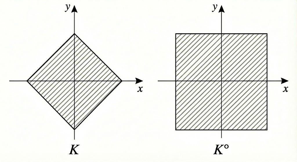

The norm induced by the polar body corresponds to the dual norm: \[ \norm{y}^*_K\defeq \norm{y}_{K^{\circ}} = \sup_{x:\norm{x}_K\leq 1} \inner{x}{y} = \sup_{x\in K} \inner{x}{y}. \] Therefore, the polar body can be defined in an alternative way as $K^\circ = \set{y: \norm{y}_K^* \leq 1}$.

Dual Sudakov’s inequality

We can now introduce the dual version of Sudakov’s inequality. While Sudakov’s inequality bounds the covering number of $T$ using balls, the dual Sudakov’s inequality bounds the covering number of the Euclidean ball using the polar of $T$.

Theorem 2 (Dual Sudakov’s inequality) For any convex set $T\subseteq \bb R^n$, \[ w(T) \gtrsim \sup_{\eps>0} \eps\sqrt{\log N(B_2^n,\eps T^\circ)}, \] where $N(B_2^n,\eps T^\circ)$ is the smallest number of translates of $\eps T^\circ$ needed to cover the Euclidean unit ball $B_2^n$.

The proof relies on a powerful “shifted measure” argument. We first establish a lemma connecting the probability mass of a set to the covering number.

Lemma 3 Let $A\in \bb R^n$ be a symmetric and convex set. If the Gaussian measure satisfies $\Pr[g\sim \+N(0,I_n)]{g\in A}\geq \frac{2}{3}$, then \[ \sup_{\eps>0}\eps\sqrt{\log N(B_2^n,\eps A)} \lesssim 1. \]

Proof. We use a volumetric argument adapted to the Gaussian measure. Let $x \in \mathbb{R}^n$. We compare the measure of a shifted set $x+A$ to the original set $A$. We have \[ \begin{align*} \Pr{g\in x+A} &= \frac{1}{(2\pi)^{\frac{n}{2}}}\cdot \int_A e^{-\frac{\norm{y+x}^2}{2}} \dd y\\ &= \frac{1}{(2\pi)^{\frac{n}{2}}}\cdot \int_A e^{-\frac{\norm{y}^2}{2}}\cdot e^{-\frac{\norm{x}^2}{2}} \cdot e^{-\inner{x}{y}}\dd y\\ &= e^{-\frac{\norm{x}^2}{2}} \cdot \E{e^{-\inner{x}{g}}\cdot \*1[g\in A]}\\ \mr{Jensen's inequality} &\geq e^{-\frac{\norm{x}^2}{2}} \cdot \Pr{g\in A}\cdot e^{-\E{\inner{x}{g}\mid g\in A}} \\ \mr{$A$ is symmetric}&=e^{-\frac{\norm{x}^2}{2}}\cdot \Pr{g\in A}. \end{align*} \]

Assume $x_1,\dots,x_p\in B_2^n$ form the maximal $\eps$-packing of $B_2^n$ with regard to $\norm{\cdot}_A$. This means the sets $x_i + \frac{\varepsilon}{2}A$ are disjoint. Considering the total probability, \[ \begin{align*} 1&\geq \Pr{g\in \bigcup_{i=1}^p \tp{\frac{2}{\eps}x_i + A}}\\ &= \sum_{i=1}^p \Pr{g\in \frac{2}{\eps}x_i + A}\\ &\geq \sum_{i=1}^p e^{-\frac{2\norm{x_i}^2}{\eps^2}}\Pr{g\in A}\\ &\geq e^{-\frac{2}{\eps^2}}\cdot p\cdot \Pr{g\in A}. \end{align*} \] This indicates \[ N(B_2^n,\eps A) \leq p\leq \frac{e^{\frac{2}{\eps^2}}}{\Pr{g\in A}}\lesssim e^{\frac{2}{\eps^2}}. \]

To prove the dual Sudakov’s inequality, we simply need to find a set $A$ related to $T^\circ$ that captures most of the Gaussian mass. Recall that $\|g\|_{T^\circ} = \sup_{t \in T} \inner{g}{t}$. By definition, $\E{\norm{g}_{T^\circ}} = w(T)$. By Markov’s inequality, \[ \begin{align*} \Pr{g\not \in 3w(T)\cdot T^\circ} &= \Pr{\norm{g}_{T^\circ} \geq 3w(T)}\\ &\leq \frac{\E{\norm{g}_{T^\circ}}}{3w(T)}\\ &\leq \frac{1}{3}. \end{align*} \] Thus, applying the above lemma with $A = 3w(T) T^\circ$, \[ \sup_{\delta>0} \delta\cdot \sqrt{\log N\tp{B_2^n, \delta\cdot 3w(T)T^{\circ}}} \lesssim 1. \] Let $\eps = \delta \cdot 3w(T)$. Substituting $\delta = \frac{\eps}{3w(T)}$, we have the dual Sudakov’s inequality \[ \sup_{\eps>0} \eps\cdot \sqrt{\log N\tp{B_2^n, \eps T^{\circ}}} \lesssim w(T). \]

Covering lemma via dual Sudakov’s inequality

Before we proceed to the proof of the primal Sudakovs’ inequality, we first see the power of the dual Sudakov’s inequality. It allows us to give a one-line proof of the covering lemma introduced in the previous lecture.

Lemma 4 (Covering lemma) Let $U \in \mathbb{R}^{M \times n}$ be a matrix with rows $u_1^\top, \dots, u_M^\top$. Define the distance \[ d_U(x,y) = \norm{U(x-y)}_{\infty} = \max_{k \in [M]} |\langle u_k, x-y \rangle|. \] Then the covering number of the Euclidean unit ball $B_2^n$ satisfies \[ \log N\tp{B_2^n, d_U, \eps}\leq \frac{\log M}{\eps^2}\cdot \max_{k\in[M]}\norm{u_k}^2_2. \]

Let us define a norm on $\mathbb{R}^n$ by $\|v\| \defeq \|Uv\|_{\infty}$. The unit ball of this norm is the set $T^{\circ} = \{x : \|Ux\|_\infty \leq 1\}$. The covering number $N(B_2^n, d_U, \varepsilon)$ is equivalent to the smallest number of translates of the scaled body $\varepsilon T^{\circ}$ needed to cover $B_2^n$. That is, \[ N(B_2^n, d_U, \eps) = N(B_2^n, \eps T^{\circ}). \] The dual Sudakov’s inequality gives that for any $\eps>0$, \[ \begin{align*} \eps \sqrt{\log N\tp{B_2^n, \eps T^{\circ}}} &\lesssim \E{\norm{g}_{T^\circ}} = \E{\norm{Ug}_{\infty}} \\ &= \E{\max_{k\in [M]} \inner{u_k}{g}} \leq \max_{k\in[M]} \norm{u_k}_2 \cdot \sqrt{\log M}. \end{align*} \] This proves the covering lemma.

From the dual Sudakov’s inequality to the primal Sudakov’s inequality

We now show how to recover the Sudakov’s inequality by a recursive argument.

First, we claim that it suffices to prove the theorem for the specific case where $X_t = \langle g, t \rangle$ for a subset $T \subset \mathbb{R}^n$, equipped with the Euclidean metric. For any $u_1,\dots,u_k\in T$, let $\Sigma$ be the covariance of $X_{u_1},\dots, X_{u_k}$. We know that $\Sigma$ can be decomposed as $AA^{\top}$ where $A=\left[t_1\ \cdots\ t_k\right]^{\top}$. The vectors $t_1,\dots,t_k$ satisify that $\inner{t_i}{t_j} = \E{X_{u_i}X_{u_j}}$. The process $\set{\inner{g}{t_i}}_{i\in[k]}$ then has the exact same distribution as $\set{X_{u_i}}_{i\in[k]}$. Furthermore, the distance is preserved: \[ d(u_i, u_j) = \sqrt{\E{(X_{u_i} - X_{u_j})^2}} = \sqrt{\|t_i\|^2 + \|t_j\|^2 - 2\langle t_i, t_j \rangle} = \|t_i - t_j\|_2. \] Therefore, we will only consider the process with the form $X_t = \langle g, t \rangle$ for some set $T\subseteq \bb R^n$.

Furthermore, we can assume without loss of generality that the set $T$ is convex and symmetric. If $T$ is not convex, we can consider its convex hull $T'$. It is easy to verify that $w(T')=w(T)$ and $N(T,d,\eps)\leq N(T',d,\eps)$. Similarly, if $T$ is not symmetric, we consider its symmetrization $T'' = T-T$. We can also prove that $w(T'') \approx w(T)$ and $\log N(T,d,\eps) \approx \log N(T'',d,\eps)$. Thus, we can assume $T$ is symmetric about the origin.

It remains to prove that \[ \log N(T,d,\eps) \lesssim \log N(B_2^n, \varepsilon T^\circ). \] Intuitively, packing Euclidian balls of radius $\eps$ into $T$ is geometrically dual to packing polars of size $\eps$ into the ball. Note that for any $x\in \bb R^n$, $\norm{x}_2^2\leq \norm{x}_T \norm{x}_{T^\circ}$. Therefore, if $\norm{x}_T \leq 2$ and $\norm{x}_{T^{\circ}}\leq \frac{\eps^2}{2}$, then $x\in \eps B_2^n$. This indicates \[ \begin{align*} N(T,\eps B_2^n) &\leq N\tp{T, 2T \cap \frac{\eps^2}{2} T^{\circ}} \\ \mr{$T\subseteq 2T$} &= N\tp{T, \frac{\eps^2}{2} T^{\circ}}\\ &\leq N(T,2\eps B_2^n) \cdot N\tp{2\eps B_2^n,\frac{\eps^2}{2} T^{\circ}}. \end{align*} \]

Taking logarithm of both sides and applying the dual Sudakov’s inequality, \[ \begin{align*} \log N(T,d,\eps) &= \log N(T, \eps B_2^n) \leq \log N(T, 2\eps B_2^n) + \log N\tp{B_2^n, \frac{\eps}{4} T^\circ} \\ &\lesssim \log N(T, 2\eps B_2^n) + \frac{w(T)^2}{\eps^2}. \end{align*} \] Solving this recursion formula yields the primal Sudakov’s inequality: \[ w(T) \gtrsim \varepsilon \sqrt{\log N(T,d,\eps)}. \] This completes the proof.