Lecture 4: Discrete Markov chains

Discrete Markov chains

Markov processes are a vital class of stochastic models used to describe a wide array of random systems. We classify these processes based on their time and state parameters. A process with discrete time steps is called a Markov chain, while the term Markov process often refers to the general case where the time can be continuous. In this note, we will focus on the most fundamental case: discrete-time Markov chains with a finite state space.

The definition

Definition 1 (Discrete Markov chain) Suppose there is a sequence of random variables \[\begin{equation*} X_0, X_1,\dots, X_t,X_{t+1},\dots \end{equation*}\] where the \(X_t \in \Omega\) for some \(\Omega\). Then we call \(\set{X_t}_{t\geq 0}\) a discrete Markov chain if \(\forall t\geq 1\) the distribution of \(X_{t}\) only depends on \(X_{t-1}\), i.e., \(\forall x_0, x_1,\dots, x_t\in \Omega\), \[\begin{equation*} \Pr{X_{t}=x_{t}|X_{t-1}=x_{t-1},\dots, X_1=x_1, X_0=x_0}=\Pr{X_{t}=x_{t}|X_{t-1}=x_{t-1}}. \end{equation*}\]

Today we will focus on the case where \(\Omega=[n]\) is finite. Then a (time-homogeneous) Markov chain can be characterized by an \(n\times n\) matrix \(P\) where \(P(i,j) = \Pr{X_{t+1}=j\mid X_{t}=i}\) for all \(t\ge 0\). We call it the transition matrix.

Such a Markov chain can be equivalently viewed as a random walk on a weighted directed graph where the edge weight from \(i\) to \(j\) equals to \(P(i,j)\).

At any time \(t\ge 0\), we use \(\mu_t\) to denote the distribution of \(X_t\), namely \[ \forall i\in [n],\quad\mu_t(i) = \Pr{X_t = i}. \] We can regard \(\mu_t\) as a vector in \([0,1]^{n}\). By the law of total probability, \(\mu_{t+1}(j) = \sum_{i} \mu_t (i) \cdot p_{ij}\) which leads to \(\mu_t^\top P = \mu_{t+1}^\top\). Consequently, we obtain \(\mu_t^\top = \mu_0^\top P^t\). As a result, the distribution at each time is entirely determined by the transition matrix \(P\) and the initial distribution \(\mu_0\). This is a useful formula as we can compute the distribution at any time given the initial distribution and the transition matrix.

Stationary distribution

A particular special distribution for a chain \(P\) is the one that remains invariant after applying \(P\).

Definition 2 (Stationary distribution) A distribution \(\pi\) is a stationary distribution of \(P\) if it remains unchanged in the Markov chain as time progresses, i.e., \[ \pi^\top P = \pi^\top. \]

The following three questions regarding stationary distributions are fundamental to Markov chains.

• Existence: does each Markov chain have a stationary distribution?
• Uniqueness: if a Markov chain has a stationary distribution, is it unique?
• Convergence: if the chain has a unique stationary distribution, does \(\mu_t\) always converge to it from any initial distribution \(\mu_0\)?

The answers to these questions are “not always,” and the conditions required to guarantee a “yes” are what make up the most important theorem in this field.

Foundamental theorem of Markov chains

First, does a stationary distribution always exist? When \(\Omega\) is finite, the answer is “yes”. This is a non-trivial result guaranteed by the Perron-Frobenius theorem, which ensures that the matrix \(P\) must have an eigenvalue of 1 with a corresponding non-negative eigenvector, which is our stationary distribution \(\pi\) (see the detailed proof in this note). This guarantee breaks down for chains with infinite state spaces. Consider a simple random walk on the integers \(\bb Z\). At each \(i\in \bb Z\), it jumps to \(i-1\) or \(i+1\) with equal probability of \(\frac{1}{2}\). Because the process does not settle into a stable, long-run behavior, it is straightforward to verify that no valid stationary distribution \(\pi\) exists.

Secondly, is the stationary distribution unique? Not always. Consider a chain with the following transition graph: If you start in the left component, you stay there forever. If you start in the right, you stay there. This chain has at least two distinct stationary distributions (e.g., being in the left component with probability 1, or being in the right with probability 1). The problem is that the chain can get “trapped.” The property that prevents this is irreducibility.

Definition 3 (Irreducibility) A finite Markov chain is irreducible if its transition graph is strongly connected.

Note that while irreducibility guarantees a unique stationary distribution, it is not a necessary condition because the distribution can have zero probability on some states. The condition becomes necessary and sufficient only when the stationary distribution is strictly positive (\(\pi_i > 0\) for all \(i\)).

For the third question, if a unique stationary distribution exists, will the chain always converge to it? Again, not necessarily. Consider the simple two-state cycle:

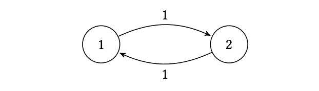
The unique stationary distribution is clearly \(\pi = (1/2, 1/2)\). However, if you start at state 1 (\(\mu_0 = (1,0)\)), the chain will be at state 1 on all even steps and state 2 on all odd steps. The distribution never settles; it oscillates between \((1,0)\) and \((0,1)\) forever. The property that prevents this deterministic cycling is aperiodicity.

Definition 4 (Aperiodicity) A Markov chain is aperiodic if for any state \(v\), it holds that \[ \gcd\set{\abs{c} \mid \ c \in C_v} = 1, \] where \(C_v\) denotes the set of the directed cycles containing \(v\) in the transition graph.

Having addressed these three issues, we can now state the important result for finite Markov chains.

Theorem 1 (Fundamental Theorem of Markov Chains, FTMC) If a finite Markov chain \(P\in\bb R^{n\times n}\) is irreducible and aperiodic, then it has a unique stationary distribution \(\pi\in\bb R^{n}\). Moreover, for any distribution \(\mu\in\bb R^n\), \[ \lim_{t\rightarrow\infty} \mu^\top P^t=\pi^\top. \]

Reversible Markov chains

We first study the FTMC for a specific class of Markov chains.

Definition 5 (Reversible Markov chains) A Markov chain \(P\) over state space \([n]\) is (time) reversible if there exists some distribution \(\pi\) satisfying \[ \forall i,j\in[n],\;\pi(i)P(i,j) = \pi(j)P(j,i). \] This equation is called the detailed balance condition.

The name reversible chain comes from the fact that for any sequence of variables \(X_0,X_1,\dots,X_t\) following the chain, the distribution of \((X_0,X_1,\dots,X_{t-1},X_t)\) is identical to the distribution of \((X_t,X_{t-1},\dots,X_1,X_0)\).

A crucial property is that this stronger condition immediately implies the standard condition for a stationary distribution.

Proposition 1 If \(P\) is reversible w.r.t a distribution \(\pi\), then \(\pi\) must be a stationary distribution of \(P\).

Proof. To see this, note that \[ \pi^\!T P(j) = \sum_{i\in[n]}\pi(i)P(i,j) = \sum_{i\in[n]}\pi(j)P(j,i) = \pi(j). \]

We will study reversible chains since their transition matrices are essentially symmetric in some sense, so many powerful tools in linear algebra apply. We will also see that reversible chains are general enough for most of our (algorithmic) applications.

Metropolis algorithms

Given a distribution \(\pi\) over a state space \(\Omega\), how can we design a Markov chain \(P\) so that \(\pi\) is the stationary distribution of \(P\)? This is equivalent to the problem of assigning transition probabilities in a transition graph \(G\) so that \(\pi\) is the stationary distribution of the random walk. The Metropolis algorithm provides a way to achieve the goal as long as \(G\) is connected and undirected.

Let’s begin with a simple random walk on a connected, non-bipartite undirected graph \(G=(V,E)\) like the following toy example.

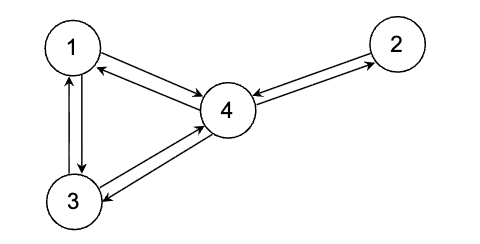
In this process, the probability of transitioning from a vertex \(i\) to an adjacent vertex \(j\) is defined as \(P(i,j) = \frac{1}{\text{deg}(i)}\), where \(\text{deg}(i)\) is the degree of \(i\). We can check the detailed balance condition and verify that its unique stationary distribution, \(\pi\), is proportional to the vertex degrees:\[\pi(i) \propto \text{deg}(i).\]

Based on this intuition, we describe the following process to construct a transition matrix \(P\) with a fixed stationary distribution \(\pi\). Let \(\Delta\) be the maximum degree of the transition graph except self-loops. That is \(\left.\Delta \triangleq \max _{u \in[n]} \sum_{v \neq u \in[n]} \mathbb{1}[(u, v) \in E]\right)\). We now assign weights to the edges. For any \(i \in[n]\), let \(\left\{v_1, v_2, \ldots, v_d\right\}\) be the \(d\) neighbours of \(i\). We consider the transition at state \(i\) :

• Choose \(k \in[\Delta+1]\) uniformly at random.
• If \(d+1 \leq k \leq \Delta+1\), do nothing.
• If \(k \leq d\), propose to move from \(i\) to \(v_k\). Then accept the proposal with probability \(\min \left\{\frac{\pi\left(v_k\right)}{\pi(i)}, 1\right\}\).

The transition matrix is, for every \(i,j\in [n]\), \[ P(i,j) = \begin{cases} \frac{1}{\Delta}\min\set{\frac{\pi(j)}{\pi(i)},1}, & \mbox{ if }i\ne j;\\ 1-\sum_{k\ne i} P(i,k), & \mbox{ if }i=j. \end{cases} \]

We can verify that \(P\) is reversible with respect to \(\pi\): for each connected \(i,j\), \[ \pi(i)P(i,j) = \pi(i)\cdot\frac{1}{\Delta}\min\set{\frac{\pi(j)}{\pi(i)},1} = \frac{\min\set{\pi(i),\pi(j)}}{\Delta} = \pi(j)P(j,i). \]

In this Metropolis algorithm, we even do not need to know \(\pi\) in order to implement the algorithm. We only need to know the quantity \(\frac{\pi(j)}{\pi(i)}\), which is much easier to compute in many applications.

We further remark that the aperiodic property is guaranteed in the above process. Note that we choose \(k \in[\Delta+1]\) rather than \([\Delta]\). This makes the chain a lazy one and thus makes the graph aperiodic.

Example 1 (Sample a proper coloring on a graph) To get a uniform sample of a proper \(q\)-colouring of a graph \(G\) with maximum degree \(\Delta\) (\(q\ge \Delta + 2\)), one can apply the Metropolis algorithm. Define the graph \(H=\tuple{V, E}\), where \(V\) is the set of all proper \(q\)-colourings, and \(E\) contains all colouring pairs that differ only at a single vertex (one can check that \(\tuple{V, E}\) is connected). Let \(\pi\) be the uniform distribution over \(V\).

We first begin with some proper colouring \(\chi_0\). At time \(t\), the transition to \(\chi_{t}\) is defined as follows:

• Select a vertex \(v \in V\) and a color \(c \in \{1, \dots, q\}\) uniformly at random.
• If recoloring \(v\) with \(c\) yields a proper coloring, accept the change. Otherwise, do nothing (\(\chi_{t} = \chi_{t-1}\)).

It is easy to verify that detailed balance condition holds for \(\pi\). That is, the uniform distribution is the stationary distribution of this Markov chain.

Spectral decomposition of reversible Markov chains

One advantage to use reversible chains is that their transition matrices have real eigenvalues. This follows from the fact that those matrices are essentially symmetric. As a result, we can apply tools in linear algebra to study them. We now develop the spectral decomposition theorem for \(P\). First, we have the following spectral decomposition theorem for symmetric \(P\).

Theorem 2 (Spectral decomposition for symmetric matrices) If \(P\in\bb R^{n\times n}\) is a symmetric matrix, then it has \(n\) real eigenvalues \(\lambda_1,\dots,\lambda_n\) with corresponding \(n\) orthonormal eigenvectors \(v_1,\dots,v_n\) satisfying \[ P = \sum_{i=1}^n\lambda_iv_iv_i^{\!T}. \] If we let \(V=\begin{bmatrix} v_1,v_2,\dots,v_n \end{bmatrix}\) and \(\Lambda = \-{diag}(\lambda_1,\dots,\lambda_n)\), then above can be written in the matrix form \[ P = V\Lambda V^\!T. \]

Without loss of generality, we assume \(\lambda_1\geq \lambda_2\geq \cdots \geq \lambda_n\). When \(P\) is a stochastic matrix with the sum of each column being \(1\), we have \(\abs{\lambda_i}\leq 1\) for each \(i\in [n]\). And because \(P \*1 = \*1\), we know that \(\lambda_1=1\).

Now we prove a similar decomposition theorem for reversible \(P\). Suppose \(P\) is reversible with respect to \(\pi\). Let \(\Pi = \-{diag}(\pi)\) be the diagonal matrix with \(\Pi(i,i) = \pi(i)\). Define \(Q=\Pi^{\frac{1}{2}}P\Pi^{-\frac{1}{2}}\), then we can verify that \(Q\) is symmetric: \[ Q(i,j) = \pi(i)^{\frac{1}{2}}P(i,j)\pi(j)^{-\frac{1}{2}} = \pi(j)^{\frac{1}{2}}P(j,i)\pi(i)^{-\frac{1}{2}} = Q(j,i). \] So we can apply the spectral decomposition theorem for \(Q\), which yields \[ Q = \sum_{i=1}^n \lambda_i u_iu_i^\!T, \] where \(\lambda_1,\dots,\lambda_n\) are eigenvalues of \(Q\) with corresponding orthonormal eigenvectors \(u_1,\dots,u_n\). If we let \(v_i\defeq \Pi^{-\frac{1}{2}}u_i\), then the above is equivalent to \[\begin{align*} P = \sum_{i=1}^n\lambda_i \Pi^{-\frac{1}{2}}u_iu_i^\!T\Pi^{\frac{1}{2}}=\sum_{i=1}^n\lambda_iv_iv_i^\!T\Pi. \end{align*}\]

We claim that \(\lambda_1,\dots,\lambda_n\) are eigenvalues of \(P\) with corresponding eigenvectors \(v_1,\dots,v_n\). To see this, we have for any \(j\in[n]\): \[\begin{align*} Pv_j &=\sum_{i=1}^n\lambda_i\Pi^{-\frac{1}{2}}u_iu_i^\!T\Pi^{\frac{1}{2}}v_j\\ &=\sum_{i=1}^n \lambda_i\Pi^{-\frac{1}{2}}u_iu_i^\!T\Pi^{\frac{1}{2}}\Pi^{-\frac{1}{2}}u_j\\ &=\lambda_jv_j. \end{align*}\] Everything looks nice if we equip \(\bb R^n\) with the inner product \(\inner{\cdot}{\cdot}_{\Pi}\) defined as \(\inner{x}{y}_\Pi = x^\!T\Pi y = \sum_{i=1}^n \pi(i)x(i)y(i)\). It is clear that \(v_1,\dots,v_n\) are orthonormal with respect to the inner product: \[ \inner{v_i}{v_j}_{\Pi} = \begin{cases} 0, & \mbox{ if }i\ne j;\\ 1, & \mbox{ if }i=j. \end{cases} \]

Variational characterization

Define the Rayleigh quotient \[ R_P(x) = \frac{\inner{\*x}{P\*x}_{\Pi}}{\inner{\*x}{\*x}_{\Pi}}. \] We can write \(\lambda_1\) as the optimum of the following optimization problem: \[ \lambda_1 = \max_{\*x\ne 0} R_{P}(\*x). \] This can be easily verified using the spectral decomposition of \(P\). Supposing \(\*x=\sum_{i=1}^n a_iv_i\), we have \[ R_P(\*x) =\frac{\sum_{i=1}^n\lambda_ia^2_i}{\sum_{i=1}^n a_i^2} = \sum_{i=1}^n \frac{a^2_i}{\sum_{j=1}^n a_j^2}\cdot\lambda_i. \]

Therefore, the Rayleigh quotient of any each nonzero \(\*x\) can be viewed as a weighted sum of all \(P\)’s eigenvalues. Of course the maximum is achieved at \(\*x=v_1\) — putting all the weight on the maximum eigenvalue. Similar arguments can be used to prove that \(\lambda_2 = \max_{\substack{\*x\ne 0\\\*x\perp v_1}} R_P(\*x)\), or more generally \[ \lambda_k = \max_{\substack{\*x\ne 0\\\*x\perp \-{span}(v_1,\dots,v_{k-1})}} R_P(\*x), \] where \(\*x\perp\*y\) means \(\inner{\*x}{\*y}_{\Pi}=0\). We can use another two-stage optimization problem to characterize \(\lambda_k\): \[ \lambda_k = \max_{\substack{k\mathrm{-dimenional\,subspace }\\V\subseteq\bb R^n}} \min_{\*x\in V\setminus\set{0}}R_P(\*x). \] To justify this, imagine the following game between two players: a max player and a min player.

• The goal of the max player is to maximize \(R_P(\*x)\), and what he can do is to provide some \(k\)-dimensional subspace \(V\subseteq\bb R^n\);
• The goal of the min player is to minimize \(R_P(\*x)\) and he can only choose those nonzero vectors from the space \(V\) provided by the max player.

Recall that for each nonzero vector \(\*x\), the value of \(R_P(\*x)\) can be viewed as a weighted sum of \(P\)’s eigenvalues. So the min players strategy must be choosing the vector whose mass is concentrated on small eigenvalues. The max player should choose the collection of vectors so that the min player’s strategy does not perform well, so his strategy must be choosing \(V=\-{span}(v_1,\dots,v_k)\). This yields the min player to choose \(\*x = c\cdot v_k\), and therefore \(R_P(\*x) = \lambda_k\).

Foundamental theorem of reversible Markov chains

Now we will give a proof of the FTMC for reversible chains using spectral decomposition. The proof is elegant, insightful and can be generalized to studying the rate of convergence.

Let us collect what we know about \(P\). First, we have the spectral decomposition \[ P = \sum_{i=1}^n\lambda_iv_iv_i^\!T\Pi = V\Lambda V^\!T\Pi, \] where \(\lambda_1\ge \lambda_2\ge\cdots\lambda_n\) are eigenvalues of \(P\) with corresponding orthonormal (w.r.t. the inner product \(\inner{\cdot}{\cdot}_{\Pi}\)) eigenvectors \(v_1,\dots,v_n\). Moreover, we know \(\lambda_1 = 1\) and \(v_1=\*1\).

With this decomposition, it is easy to compute \[ P^t = \sum_{i=1}^n \lambda_i^t v_iv_i^\!T\Pi = \*1\pi^\!T + \sum_{i=2}^n\lambda_i^t v_iv_i^\!T\Pi. \]

Note that \(\*1\pi^\!T = \begin{bmatrix}\pi^\!T\\\pi^\!T\\\vdots\\\pi^\!T\end{bmatrix}\) and therefore for any distribution \(\mu\), it holds \(\mu^\!T\*1\pi^\!T = \pi^\!T\). This implies that \[ \lim_{t\to\infty} \mu^\!TP^t = \pi^\!T + \lim_{t\to\infty}\mu^\!T\tp{\sum_{i=2}^n \lambda_i^t v_iv_i^\!T \Pi}. \] Therefore we only need to argue when \[ \lim_{t\to\infty}\mu^\!T\tp{\sum_{i=2}^n \lambda_i^t v_iv_i^\!T \Pi} = 0. \]

Since \(P\) is stochastic, we know that \(\abs{\lambda_i}\le 1\) for all eigenvalues \(\lambda_i\) of \(P\). Therefore, there are two ways to prohibit \(\lim_{t\to\infty}\mu^\!T\tp{\sum_{i=2}^n \lambda_i^t v_iv_i^\!T \Pi} = 0\), \(\lambda_2=1\) or \(\lambda_n = -1\). We will now show that the two cases correspond to reducibility and periodicity of \(P\) respectively.

Since we assume \(P\) is reversible, all edges in \(P\) can be viewed as being undirected, namely \((u,v)\in E\iff (v,u)\in E\). As a result, reducibility is equivalent to that the transition graph is disconnected.

We now prove

Proposition 2 \(\lambda_2=1\) if and only if the transition graph of \(P\) is disconnected.

Proof. The main tool to prove the proposition is the variational characterization of eigenvalues. Recall that \[\begin{align*} \lambda_2 &=\max_{\substack{\*x\ne 0\\\*x\perp\*1}} R_{P}(\*x)\\ &=\max_{\substack{\*x\ne 0\\\*x\perp\*1}} \frac{\inner{\*x}{P\*x}_{\Pi}}{\inner{\*x}{\*x}_{\Pi}}\\ &=\max_{\substack{\*x\ne 0\\\*x\perp\*1}} \frac{\sum_{(i,j)\in V^2}\pi(i)P(i,j)x(i)x(j)}{\sum_{i\in V}\pi(i)x(i)^2} + 1 - 1\\ &=\max_{\substack{\*x\ne 0\\\*x\perp\*1}} 1-\frac{\sum_{\set{i,j}\in E}\pi(i)P(i,j)(x(i)-x(j))^2}{\sum_{i\in V}\pi(i)x(i)^2} \end{align*}\] Therefore, \(\lambda_2=1\) if and only if we can find some nonzero \(\*x\perp \*1\) such that \(\frac{\sum_{\set{i,j}\in E}\pi(i)P(i,j)(x(i)-x(j))^2}{\sum_{i\in V}\pi(i)x(i)^2}=0\). Clearly this is equivalent to that \(P\) is disconnected.

In fact, we can prove that \(\lambda_k=1\) iff \(P\) contains at least \(k\) connected components.

Note that when \(P\) is reversible and irreducible, every edge is part of a 2-cycle (\(i \to j \to i\)), Then the chain is aperiodic if and only if its graph contains at least one odd-length cycle, which indicates that aperiodicity is equivalent to the underlying graph being non-bipartite. We can prove the following property.

Proposition 3 \(\lambda_n=-1\) if and only if the transition graph of \(P\) is bipartite.

Proof. Again by the variational characterization of \(\lambda_n\), we have \[\begin{align*} \lambda_n &=\min_{\*x\ne 0}R_{P}(\*x)\\ &=\min_{\*x\ne 0}\frac{\sum_{(i,j)\in V^2}\pi(i)P(i,j)x(i)x(j)}{\sum_{i=1}^n\pi(i)x(i)^2}+1-1\\ &=\min_{\*x\ne 0}\frac{\sum_{(i,j)\in V^2}\pi(i)P(i,j)x(i)x(j)+\sum_{(i,j)\in V^2}\pi(i)P(i,j)x(i)^2}{\sum_{i=1}^n\pi(i)x(i)^2} - 1\\ &=\min_{\*x\ne 0}\frac{2\sum_{(i,j)\in V^2}\pi(i)P(i,j)x(i)x(j)+\sum_{(i,j)\in V^2}\pi(i)P(i,j)(x(i)^2+x(j)^2)}{2\sum_{i=1}^n\pi(i)x(i)^2} - 1\\ &=\min_{\*x\ne 0}\frac{\sum_{(i,j)\in V^2}\pi(i)P(i,j)(x(i)+x(j))^2}{2\sum_{i=1}^n\pi(i)x(i)^2} - 1 \end{align*}\] Clearly the numerator is zero for some nonzero \(\*x\) if and only if \(P\) is bipartite.

Coupling

As mentioned in the class, a Markov chain can be viewed in many different ways: as a stochastic process, or a linear operator, or as a matrix, among others. Each perspective offers its own tool to prove the FTMC. In the following part of this lecture, we will employ the method of coupling, a technique widely used in probability theory.

It will become clear later that coupling is closely related to the total variation distance between two distributions.

Definition 6 (Total Variation Distance) The total variation distance between two distributions \(\mu\) and \(\nu\) on a countable state space \(\Omega\) is given by \[ D_{\!{TV}}(\mu, \nu) = \frac12 \sum_{x\in \Omega} \abs{\mu(x) - \nu(x)}. \]

We can look at the following figure (for pdf) of two distributions on the same sample space. The total variation distance is half the area enclosed by the two curves.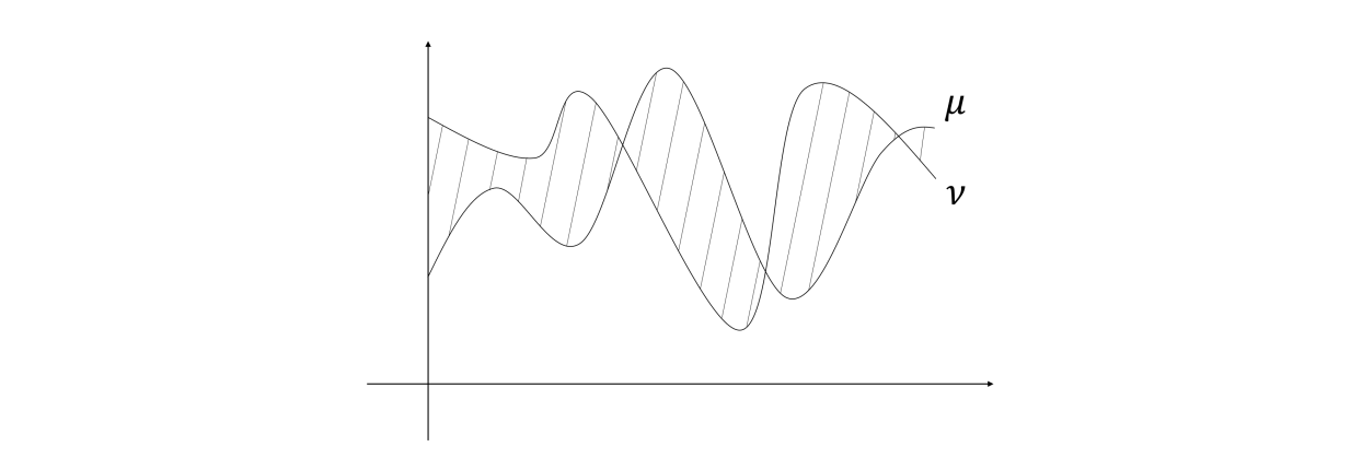

This figure immediately implies the following proposition.

Proposition 4 We define \(\mu(A) = \sum\limits_{x\in A} \mu(x)\), \(\nu(A) = \sum_{x\in A}\nu(x)\), then we have \[\begin{align*} D_\!{TV}(\mu, \nu) = \max _{A \subseteq \Omega} \abs{\mu(A) - \nu(A)}. \end{align*}\]

We can compare two distributions using couplings. The method finds numerous applications in probability theory.

A coupling of two distributions is simply a joint distribution of them.

Definition 7 (Coupling) Let \(\mu\) and \(\nu\) be two distributions on the same space \(\Omega\). Let \(\omega\) be a distribution on the space \(\Omega \times \Omega\). If \((X, Y) \sim \omega\) satisfies \(X \sim \mu\) and \(Y \sim \nu\), then \(\omega\) is called a coupling of \(\mu\) and \(\nu\).

In other words, the marginal probabilities of the disjoint distribution \(\omega\) are \(\mu\) and \(\nu\) respectively. A special case is when \(x\) and \(y\) are indepent. However, in many applications, we want \(x\) and \(y\) to be correlated while keeping their respect marginal probabilities correct.

We now give a toy example about how to construct different couplings on two fixed distributions. There are two coins: the first coin has probability \(\frac{1}{2}\) for head in a toss and \(\frac{1}{2}\) for tail, and the second coin has probability \(\frac{1}{3}\) and \(\frac{2}{3}\) respectively. We now construct two couplings as follows.

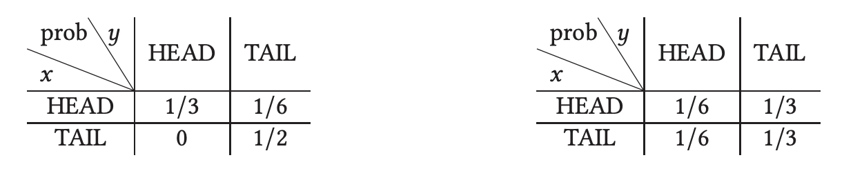
The table defines a joint distribution and the sum of a certain row/column equal to the corresponding marginal probability. It is clear that both table are couplings of the two coins. Among all the possible couplings, sometimes we are interested in the one who is “mostly coupled”.

Lemma 1 (Coupling Lemma) Let \(\mu\) and \(\nu\) be two distributions on a sample space \(\Omega\). Then for any coupling \(\omega\) of \(\mu\) and \(\nu\) it holds that, \[\begin{align*} \Pr[(X,Y)\sim \omega]{X \neq Y} \geq D_\!{TV}(\mu, \nu). \end{align*}\] And furthermore, there exists a coupling \(\omega^*\) of \(\mu\) and \(\nu\) such that \[\begin{align*} \Pr[(X,Y)\sim\omega^*]{X \neq Y} = D_\!{TV}(\mu, \nu). \end{align*}\]

Proof. For finite \(\Omega\), designing a coupling is equivalent to filling a \(\Omega \times \Omega\) matrix in the way that the marginals are correct.

Clearly we have \[\begin{align*} \Pr{X = Y} & = \sum_{t \in \Omega} \Pr{X = Y = t} \\ & \leq \sum_{t \in \Omega} \min\set{\mu(t), \nu(t)}. \end{align*}\] Thus, \[\begin{align*} \Pr{X \neq Y} & \geq 1 - \sum_{t \in \Omega} \min\tp{\mu(t),\nu(t)} \\ & = \sum_{t \in \Omega} \left(\mu(t) - \min\set{\mu(t), \nu(t)}\right) \\ & = \max_{A \subseteq \Omega} \set{\mu(A) - \nu(A)} \\ & = D_\!{TV}(\mu, \nu). \end{align*}\] To construct \(\omega^*\) achieving the equality, for every \(t\in\Omega\), we let \(\Pr[(X,Y)\sim\omega^*]{X = Y = t} = \min\set{\mu(t), \nu(t)}\).

Example 2 Consider two Erdős-Rényi random graphs \(G(n, p)\) and \(G(n,q)\) with \(0\leq p\leq q\leq 1\). We now wish to prove this intuitive result: \[ \mathbb{P}_{G \sim G(n, p)}[G \text{ is connected}] \le \mathbb{P}_{H \sim G(n, q)}[H \text{ is connected}] \] While this seems obvious—more edges should increase the likelihood of connectivity—a rigorous proof is not immediately apparent. We can demonstrate this elegantly using the technique of coupling.

First, let’s consider a practical way to sample from \(G(n, p)\) and \(G(n, q)\) simultaneously. For each pair \(\{i, j\}\), we will draw a uniform random number \(r_{ij}\) and use it to determine the edge’s existence in both graphs: * The edge \(\{i, j\}\) is in \(G\) if \(r_{ij} \le p\). * The edge \(\{i, j\}\) is in \(H\) if \(r_{ij} \le q\).

This joint construction defines a coupling, which we can call \(\omega\), of the two distributions. Crucially, this setup guarantees that if an edge \(\{i, j\}\) exists in \(H\), then it is also in \(G\). In other words, \(G\) is always a subgraph of \(H\). This leads directly to our conclusion. If the graph \(G\) is connected, then the graph \(H\) (which contains all of \(G\)’s edges and possibly more) must also be connected. Therefore,
\[\begin{align*} \mathbb{P}_{G \sim G(n, p)}[G \text{ is connected}] &= \mathbb{P}_{(G, H) \sim \omega}[G \text{ is connected}] \\ &\le \mathbb{P}_{(G, H) \sim \omega}[H \text{ is connected}] \\ &= \mathbb{P}_{H \sim G(n, q)}[H \text{ is connected}]. \end{align*}\]

Coupling of two Markov chains

Assume the Markov chain \(P\) has a stationary distribution \(\pi\). To prove the FTMC, what we would like to show is that for all starting distribution \(\mu_0\), it holds that \[ \lim_{t\to\infty} D_{\!{TV}}(\mu_t,\pi) = 0\,, \] where \(\mu_t^\!T = \mu_0^\!T P^t\). We will not discuss the detailed proof of the FTMC via coupling of Markov chains in this lecture. Nevertheless, the method itself is a powerful technique. We will now introduce the idea and some applications.

Suppose that \(\{X_t\}\) and \(\{Y_t\}\) are two identical Markov chains starting from different distribution, where \(Y_0\sim \pi\) while \(X_0\) is generated from an arbitrary distribution \(\mu_0\).

Now we have two sequence of random variables: \[\begin{align*} \begin{array}{*{13}{c}} \mu_0 & & \mu_1 & & & & & & \mu_t & & & & \cr \wr & & \wr & & & & & & \wr & & & & \cr X_0 & \to & X_1 & \to & X_2 & \to & \cdots & \to & X_t & \to & X_{t + 1} & \to & \cdots\cr & & & & & & & & & & & & \cr Y_0 & \to & Y_1 & \to & Y_2 & \to & \cdots & \to & Y_t & \to & Y_{t + 1} & \to & \cdots\cr \wr & & \wr & & & & & & \wr & & & & \cr \pi & & \pi & & & & & & \pi & & & & \end{array} \end{align*}\] The coupling lemma establishes the connection between the distance of distributions and the discrepancy of random variables. To show that \(D_{\!{TV}}(\mu_t,\pi) \to 0\), it is sufficient to construct a coupling \(\omega_t\) of \(\mu_t\) and \(\pi\) and then compute \(\Pr[(X_t,Y_t)\sim \omega_t]{X_t \neq Y_t}\).

Mixing time

This technique can be used to analyse the mixing time of Markov chains. For any \(\eps>0\), the mixing time of a Markov chain \(P\) up to error \(\eps\) is the minimum step \(t\) such that if we run the Markov chain from any initial distribution, its total variation distance to the stationary distribution is at most \(\eps\). Formally, \[\begin{equation*} \tau_{\!{mix}}(\eps):=\min_{t}\max_{\mu_0} D_{\-{TV}}(\mu_t,\pi)\le \eps. \end{equation*}\]

Example 3 (Random walk on the hypercubes) Consider the random walk on the \(n\)-cube. The state space \(\Omega = \{0, 1\}^n\), and there is an edge between two state \(x\) and \(y\) iff \(\|x-y\|_1=1\). We start from a point \(X_0 \in \Omega\). In each step,

• With probability \(\frac 12\) do nothing.
• Otherwise, pick \(i\in[n]\) uniformly at random and flip \(X(i)\).

It’s equivalent to the following process:

• Pick \(i\in[n], c \in \{0, 1\}\) uniformly at random.
• Change \(X(i)\) to \(c\).

Now we analyze the mixing time of the process using coupling. We apply the following simple coupling rule:

The two walks \(X_t\) and \(Y_t\) choose the same \(i, c\) in every step.

Once a position \(i\in [n]\) has been picked, \(X_t(i)\) and \(Y_t(i)\) will be the same forever. Therefore, the problem again reduces to the coupon collector problem. For \(t\geq n\log n + cn\), the probability that the \(i^{th}\) dimension is not chosen is \[\begin{equation*} \tp{1-\frac{1}{n}}^{n\log n + cn}\leq \frac{e^{-c}}{n}. \end{equation*}\] Then the probability that there exists at least one dimension which is not chosen is no larger than \(e^{-c}\). We want this value to be less than \(\epsilon\). Then we choose \(c>\log \frac{1}{\epsilon}\). Thus, \[ \tau_{\!{mix}}(\eps) \le n\log\frac{n}{\eps}. \]

Example 4 (Shuffling cards) Given a deck of \(n\) cards, consider the following rule of shuffling

• pick a card uniformly at random;
• put the card on the top.

The shuffling rule can be viewed as a random walk on all \(n!\) permutations of the \(n\) cards and it is easy to verify that the uniform distribution is the stationary distribution. Let us design a coupling for this Markov chain. That is, let \(X_t\) and \(Y_t\) be decks of cards, and we construct \(X_{t+1}\) and \(Y_{t+1}\) by

picking the same card

Note that we are picking the ``same card’’, not the card at the same location. In other words, once we pick \(\heartsuit K\) in \(X_t\), we pick \(\heartsuit K\) in \(Y_t\) as well.

This is clearly a coupling, and once some card, say \(\heartsuit K\) has been picked, then \(\heartsuit K\) in two decks will be always at the same location. Therefore, if we ask in how many rounds \(T\), \(X_T=Y_T\), the question is equivalent to the coupon collector problem again. So we have, \[ \tau_{\-{mix}}(\eps) \le n\log\frac{n}{\eps}. \]

Relaxation time

The mixing time defined above is closely related to the notions when we analyse the Markov chains in the view of linear algebra. By discussion above, if \(\lambda_2<1\) and \(\lambda_n>-1\), or equivalently \(P\) is aperiodic and irreducible, then \[ \lim_{t\to\infty}\mu^\!T\tp{\sum_{i=2}^n \lambda_i^t v_iv_i^\!T \Pi} = 0. \] The gap between \(1\) and the absolute value of these two eigenvalues also determines how fast \(P^t\) converges to \(\*1\pi^{\!T}\).

Let \(\lambda^*\defeq \max\set{\abs{\lambda_2},\abs{\lambda_n}}\), then the relaxation time of \(P\) is defined to be \[ \tau_{\-{rel}}\defeq \frac{1}{1-\lambda^*}. \]

It measures the rate of convergence and is related to the mixing time as follows:

Theorem 3 Let \(P\) be a reversible chain with stationary distribution \(\pi\), then \[ (\tau_{\-{rel}}-1)\log\frac{1}{2\eps} \le \tau_{\-{mix}}(\eps) \le \tau_{\-{rel}}\log\frac{1}{\eps\pi_{\-{min}}}, \] where \(\pi_{\-{min}}=\min_{x\in\Omega}\pi(x)\).