Lecture 5: Geometry View of Markov Chains, Brownian motion

Author

instructed by Chihao Zhang, scribed by Jinxuan Zhu and Yuchen He

Geometry View of Markov Chains

Graph expansion

Consider a simple random walk on a graph where, at each step, one moves to a neighbor chosen uniformly at random. The transition probability \(P(i,j)=\frac{1}{\deg(i)}\) if \((i,j)\) is an edge, and its stationary distribution \(\pi\) is proportional to the vertex degrees: \(\pi(i) \propto \deg(i)\).

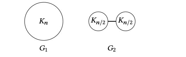
The mixing time is highly dependent on the graph’s structure. For example, on the complete graph \(K_n\), the walk mixes in one step. Conversely, on a graph with a bottleneck (e.g., two large cliques connected by a single edge), mixing is very slow, as all probability flow between the large parts must pass through that bottleneck.

Let \(P\) be a reversible chain on \(\Omega\). For any \(i,j \in \Omega\), define the probability flow from \(i\) to \(j\) as \(Q(i,j)\defeq \pi(i)P(i,j)\). Similarly, for any \(S\subset \Omega\), the flow from \(S\) to \(\bar{S}\), denoted by \(Q(S,\bar S)\), is \(\sum_{i\in S, j\in \Omega\setminus S}Q(i,j)\), and we define the expansion of \(S\) as \[ \Phi(S) = \frac{Q(S,\bar{S})}{\pi(S)}, \] where \(\pi(S)=\sum_{i\in S}\pi(i)\).

If \(X_t\sim\pi\), a direct calculation shows that the expansion of a set \(S\) is the probability of leaving that set in one step: \[ \Phi(S) = \Pr{X_{t+1}\not\in S\mid X_t\in S}. \]

The expansion of the entire chain \(P\) is defined as the minimum expansion over all sets with measure at most \(1/2\): \[ \Phi(P) = \min_{S\subseteq \Omega:\pi(S)\le \frac{1}{2}}\Phi(S). \]

The following theorem justifies our intuition that small expansion (i.e., a bottleneck) implies slow mixing.

Theorem 1 Let \(P\) be a reversible chain. \[\tau_{mix}(\eps)\ge \frac{1-2\eps}{2} \frac{1}{\Phi(P)}.\]

Proof. Let \(\{X_t\}_{t \ge 0}\) be a Markov chain generated by \(P\) and \(X_0 \sim \pi\). Let \(S=\argmin_{\pi(S)\le \frac{1}{2}} \Phi(S)\). Then \[\begin{align*} \Pr{X_t\in \bar{S}\mid X_0 \in S} &= \frac{\Pr{X_t\in \bar{S} \land X_0\in S}}{\Pr{X_0\in S}}\\ &\le \frac{\sum_{i=0}^{t-1} \Pr{X_i\in S\land X_{i+1}\in \bar{S}}}{\Pr{X_0\in S}}\\ &= \frac{t \cdot\Pr{X_1\in \bar{S} \land X_0\in S}}{\Pr{X_0\in S}}\\ &= t\cdot \Pr{X_1\in \bar{S}\mid X_0\in S}\\ &= t\cdot \Phi(S). \end{align*}\] So there exists \(x_0\) such that \[\begin{align*} \Pr{X_t\in S\mid X_0=x_0} \geq 1-t\cdot \Phi(S). \end{align*}\] Therefore, \[ D_{\!{TV}}(P^t(x_0, \cdot),\pi)\geq 1-t\cdot \Phi(S)-\pi(S) \geq \frac{1}{2}-t\cdot \Phi(S)\geq \eps,\] as long as \(t \leq \frac{1-2\eps}{2} \frac{1}{\Phi(P)}\).

Applications for Sampling Colorings

Assume we want to sample from all proper \([q]\)-colorings on \(G=([n],E)\) with maximum degree \(\Delta\). The Markov chain is

Pick \(v\in [n]\) and \(c\in [q]\) uniformly at random.
Recolor \(v\) with \(c\) if possible.

Recall that we proved \(\tau_{mix}(\eps)\leq q n \log \frac{n}{\eps}\) when \(q>4\Delta\). Now we want to argue that when \(q\) is rather small, the expansion is large for some special graph.

Consider the case when \(G\) is a star and \(1\) is the vertex at the center. Let \(Z\) be the number of all proper colorings on \(G\), and \(S\) be the set of proper colorings that the color of \(1\) is \(1\). Then we have \[\begin{align*} Q(S,\bar{S})&=\sum_{i\in S, j\in \bar{S}} \pi(i)P(i,j)\\ &=(q-1)(q-2)^{n-1}\frac{1}{Z\cdot nq}. \end{align*}\] Since \(|S|=(q-1)^{n-1}\), we have \[ \Phi(S)=\frac{Q(S,\bar{S})}{\pi(S)}=\frac{(q-2)^{n-1}}{(q-1)^{n-2}}\frac{1}{nq}=\frac{q-1}{nq}\tp{1-\frac{1}{q-1}}^{n-2}\le \frac{1}{n} \exp\tp{-\frac{n-2}{q-1}}. \] Therefore, \(\tau_{mix}=\Omega\tp{n\cdot \exp\tp{\frac{q-1}{n-2}}}\), which means that when \(q=o(\frac{n}{\log n})\), \(\tau_{mix}\) is \(n^{\omega(1)}\).

Cheeger’s inequality

We have previously established a relationship between mixing time and expansion, bridging the probabilistic and geometric perspectives of the chain. We now introduce Cheeger’s inequality, which connects expansion with eigenvalues. This inequality bridges the geometric and algebraic viewpoints.

Sometimes it is more convenient to work with \(L=I-P\), the Laplacian of \(P\). Then \[ L=\sum_{i=1}^n(1-\lambda_i)\*v_i\*v_i^{\!T}\Pi. \] For every \(i=1,2,\dots,n\), we use \(\gamma_i\) denote \(1-\lambda_i\). Then \(0=\gamma_1\le\gamma_2\le\cdots\le\gamma_n\le 2\) are the eigenvalues of \(L\).

The Cheeger’s inequality is \[ \frac{\gamma_2}{2}\le\Phi(P)\le \sqrt{2\gamma_2}. \]

We use the tool of Rayleigh quotient to prove this. For the matrix \(L\), the Rayleigh quotient is defined as \[ R_L(x) := \frac{\langle x, L x \rangle_\pi}{\langle x, x \rangle_\pi} \]

Expanding the expression yields a useful representation for \(R_L(x)\):

\[\begin{align*} R_L(x) &= \frac{\langle x, L x \rangle_\pi}{\langle x, x \rangle_\pi} \\ &= \frac{\sum_{i=1}^n x_i \pi_i ( x_i - \sum_{j=1}^n P_{ij} x_j )}{\sum_{i=1}^n x_i \pi_i x_i} \\ &= \frac{\sum_{i=1}^n x_i^2 \pi_i - \sum_{i,j\in [n]} \pi_i P_{ij} x_i x_j}{\sum_{i=1}^n \pi_i x_i^2} \\ &=\frac{\frac{1}{2} \sum_{i,j\in [n]} \pi_i P_{ij} (x_i - x_j)^2}{\sum_{i=1}^n \pi_i x_i^2} \\ &= \frac{\sum_{i,j\in [n], i<j} \pi_i P_{ij} (x_i - x_j)^2}{\sum_{i=1}^n \pi_i x_i^2}. \end{align*}\]

This formula reveals that the Rayleigh quotient measures how much the vector \(x\) varies over the state space relative to the chain’s transition structure. A small \(R_L(x)\) indicates that \(x\) is a “smooth” vector, assigning similar values to highly connected states. Conversely, a large \(R_L(x)\) signals that the values of \(x\) change sharply across the graph’s edges.

Proof of \(\gamma_2\le 2\Phi(P)\)

Recall that \[ \gamma_2 = \min_{2-\-{dim}\,V\subseteq \^R^n }\max_{x\in V\setminus\set{\*0}} R_L(\*x). \] Therefore, in order to prove an upper bound for \(\gamma_2\), it suffices to construct some \(2\)-dimensional space \(V\) such that any nonzero \(\*x\in V\) has small \(R_L(\*x)\).

Suppose \(\Phi(P)=\Phi(S)\) for some \(S\subseteq V\). Let \(\*1_S\) and \(\*1_{\ol S}\) be the indicator vector of \(S\) and its complement \(\ol{S}\) respectively. Consider the space \(V=\-{span}(\*1_S,\*1_{\ol S})\). Then every \(\*x\in V\) can be written as \(\*x=a\*1_S + b\*1_{\ol S}\) for some \(a,b\in\^R\). We have \[\begin{align*} R_L(a\*1_S) &= \frac{\sum_{i\in S,j\in\ol{S}}\pi(i)P(i,j)}{\pi(S)}\\ &= \frac{\sum_{i\in S, j\in\ol{S}}\Pr{X_t=i\land X_{t+1}=j}}{\pi(S)}\\ &=\frac{\Pr{X_t\in S\land X_{t+1}\in\ol{S}}}{\pi(S)}\\ &=\Phi(S). \end{align*}\] Similarly, we have \(R_L(b\*1_{\ol{S}}) = \Phi(\ol{S})\).

The inequality then follows from the following proposition:

Proposition 1 If at least one of \(\*x\) and \(\*y\) is not zero, then \(R_L(\*x+\*y)\le 2\max\set{R_L(\*x),R_L(\*y)}\).

Proof. Assume \(\*x=\sum_{i=1}^n a_i\*v_i\) and \(\*y=\sum_{i=1}^n b_i\*v_i\). Then \[\begin{align*} R_L(\*x+\*y) &=\frac{\inner{\*x+\*y}{L(\*x+\*y)}_{\Pi}}{\inner{\*x+\*y}{\*x+\*y}_{\Pi}}\\ &=\frac{\sum_{i=1}^n(a_i+b_i)^2\lambda_i}{\sum_{i=1}^n(a_i+b_i)^2}\\ &\le \frac{2\sum_{i=1}^n(a_i^2+b_i^2)\lambda_i}{\sum_{i=1}^na_i^2+b_i^2}\\ &\le 2\cdot\max\set{R_L(\*x),R_L(\*y)}. \end{align*}\]

Proof overview of \(\Phi(P)\le \sqrt{2\gamma_2}\)

In order to prove an upper bound for \(\Phi(P)\), it is enough to find \((S,\bar{S})\) such that \(\Phi(S)\lor \Phi(\bar{S})\le \sqrt{2\gamma_2}\). We give an approximation algorithm to estimate \(\Phi(P)\) and the upper bound is a consequence of the analysis of its performance. The algorithm is called Fiedler’s Algorithm:

With input \(\Omega\) and \(\*x\in\^R^{\Omega}\). * Sort \(\Omega=\set{v_1,\dots,v_n}\) according to \(\*x\) (namely \(x(v_1)\le x(v_2)\le \dots\)); * For every \(i\in[n]\), let \(S_i=\set{v_1,v_2,\dots,v_i}\); * Return \(\min_{i\in[n]} \Phi(S_i)\lor \Phi(\ol{S}_i)\).

We prove the following stronger theorem:

Theorem 2 For all \(\*x\perp\*1\), let \(S\) be the set returned by Fiedler’s algorithm on the input \(\*x\). Then \[ \Phi(S)\le\sqrt{2R_L(\*x)}. \]

The Cheeger’s inequality then follows by taking \(\*x=\*v_2\).

For simplicity, we assume \(\Omega=[n]\) and \(\*x(1)\leq \*x(2)\leq \dots\) here. To prove the theorem, we first normalize the vector \(\*x\). Let \[ \ell \defeq \min\set{k\in[n]\mid \sum_{i=1}^k \pi(i)\ge\sum_{i=k+1}^n\pi(i)}, \] and for every \(i\in [n]\), let \(y_i = x_i - x_{\ell}\). By the definition, \(y_\ell=0\) and \(y_i\le 0\) for all \(i\le \ell\), \(y_i\ge 0\) for all \(i\ge \ell\).

We have the following proposition:

Proposition 2 \(R_L(\*x)\ge R_L(\*y)\).

Proof. To see why it holds, note that \[ R_L(\*x) = \frac{\sum_{i,j}\pi(i)P(i,j)(x_i^2-x_ix_j)}{\inner{\*x}{\*x}_{\Pi}}=\frac{\sum_{\substack{i,j\in \Omega\\i<j}}\pi(i)P(i,j)\tp{x_i-x_j}^2}{\inner{\*x}{\*x}_{\Pi}}. \] Since \(\*y = \*x - y_\ell\*1\) is obtained from \(\*x\) by substracting a constant multiples of \(\*1\), this operation does not change the numerator and increase the denominator (because \(\*x\perp \*1\)). This can also be verified via direct calculation.

As a result, we only need to prove that \(\Phi(S)\le\sqrt{2R_L(\*y)}\). We prove by the probabilistic method. That is, we randomly choose some \(t\in[y_1,y_n]\) (following a certain tailored density) and consider the expected expansions of \(\Phi(S_t)\) and \(\Phi(\ol{S}_t)\) where \(S_t\defeq\set{i\in[n]\mid y_i\le t}\).

To this end, we can normalize \(\*y\) by dividing some constant and assume without loss of generality that \(y_1^2+y_n^2=1\). We sample \(t\) with density \(p(t)=2\abs{t}\).

Note that for every \(t\in[y(1),y(n)]\), \[ \max\set{\Phi(S_t),\Phi(\ol{S}_t)} = \frac{\sum_{i\in S_t,j\in \bar{S_t}}\pi(i)P(i,j)}{\min\set{\pi(S_t),\pi(\ol{S}_t)}}=:\frac{A}{B}. \]

Via some calculations, we can prove that \[ \E{A}\leq \sqrt{2 \langle y, y \rangle_\pi} \sqrt{\langle y, L y \rangle_\pi} \] and \[ \E{B}= \langle y, y \rangle_\pi. \] For detailed proofs, see Sec 2.2 of this note. This yields \[ \frac{\E{A}}{\E{B}}\le \frac{\sqrt{2\inner{\*y}{\*y}_{\Pi}}\cdot\sqrt{\inner{\*y}{L\*y}_{\Pi}}}{\inner{\*y}{\*y}_{\Pi}} = \sqrt{2R_L(\*y)} \le \sqrt{2R_L(\*x)}. \]

Moreover, for any \(r\), we have \[ \frac{\E{A}}{\E{B}}\le r\implies \E{A-rB}\le 0 \implies \Pr{\frac{A}{B}\le r}>0. \] The Cheeger’s inequality is proved.

Brownian motion

Brownian motion describes the random movement of small particles suspended in a liquid or gas. This phenomenon was named after the botanist Robert Brown, who observed and studied the jittery movement of pollen grains suspended in water under a microscope. Later, Albert Einstein provided a physical explanation for this phenomenon. In mathematics, Brownian motion is characterized by the Wiener process, named after Norbert Wiener, a renowned mathematician and the originator of cybernetics

To motivate the definition of Brownian motion, we start from the \(1\)-D random walk starting from \(0\). Let \(Z_t\) be our position at time \(t\) and \(X_t\) be the move of the \(t\)-th step. The value of \(X_t\) is chosen from \(\set{-1,1}\) uniformly at random. Note that \(Z_0=0\) and \(Z_{t}=Z_{t-1}+X_t\) for \(t>0\). So \(Z_T=\sum_{t=1}^{T} X_t\). Then we have \[ \E{Z_T}=0\-{\ and\ }\Var{Z_T}=\sum_{t=1}^{T}\Var{X_t}=T. \]

Suppose we now move every \(\delta\) seconds, with step length \(C\). Then the position at time \(T\) is

\[ Z(T) = C \sum_{i=1}^{T / \delta} X_i, \]

with expectation and variance

\[ \E{Z(T)} = 0\ \mbox{ and }\ \Var{Z(T)} = C^2 \frac{T}{\delta}. \]

We can identify the expectation and the variance of this process with the discrete random walk when \(\delta\to 0\) by choosing \(C=\sqrt{\delta}\). It follows from the central limit theorem that \[ \lim_{\delta \to 0} Z(T) = \sqrt{T} \lim_{\delta \to 0} \frac{\sum_{i=1}^{T / \delta} X_i}{\sqrt{\frac{T}{\delta}}} \overset{D}{\to} \+N(0,T) \]

In other words, the “continuous” version of the 1-D random walk follows \(\+N(0,T)\) at time \(T\). This is the basis of the Wiener process. Now we introduce its formal definition.

Definition 1 (Standard Brownian Motion / Wiener Process) We say a stochastic process \(\set{W(t)}_{t\geq 0}\) is a standard Brownian motion or Wiener process if it satisfies

\(W(0)=0\);
Independent increments: \(\forall 0\leq t_0\leq t_1\leq \cdots\leq t_n\), \(W(t_1)-W(t_0)\), \(W(t_2)-W(t_1)\), \(\dots\), \(W(t_n)-W(t_{n-1})\) are mutually independent;
Stationary increments: \(\forall s,t>0\), \(W(s+t)-W(s)\sim \+N(0,t)\);
\(W(t)\) is continuous almost surely.

Recall the probability density function of normal distribution \(\+N(0, t)\), denoted as \(f_t(x)\), is \[ f_t(x) = \frac{1}{\sqrt{2\pi t}} \exp\left(-\frac{x^2}{2t}\right) \]

Then for any \(0 \leq t_1 \leq \cdots \leq t_n\), the joint probability density function of \(W(t_1), W(t_2), \ldots, W(t_n)\) is \[ f(x_1, \ldots, x_n) = f_{t_1}(x_1) f_{t_2 - t_1}(x_2 - x_1) \ldots f_{t_n - t_{n-1}}(x_n - x_{n-1}). \]

Gaussian process

Now we will give another characterization of Brownian motions in terms of the Gaussian process. First recall the notion of high dimensional Gaussian distribution. A vector of random variables \((X_1,X_2,\dots,X_n)\) is said to be Gaussian iff \(\forall a_1,a_2,\dots,a_n\), \(\sum_{i=1}^n a_iX_i\) is a one-dimensional Gaussian. Let \(\mu=(\mu_1,\mu_2,\dots,\mu_n)\) where \(\mu_i=\E{X_i}\). Let \(\Sigma=\tp{\-{Cov(X_i,X_j)}}_{i,j}\). Then the probability density function \(f\) of \((X_1,X_2,\dots,X_n)\) is \[ \-{for\ }x=(x_1,x_2,\dots,x_n),\ f(x)=(2\pi)^{-\frac{n}{2}}\cdot \abs{\-{det}\Sigma}^{-\frac{1}{2}}\cdot e^{-\frac{1}{2}(x-\mu)^{T}\Sigma^{-1}(x-\mu)}. \]

Definition 2 (Gaussian process) A stochastic process \(\set{X(t)}_{t\geq 0}\) is called Gaussian process if \(\forall 0\leq t_1\leq t_2\leq \dots \leq t_n\), \(\tp{X(t_1),X(t_2),\dots,X(t_n)}\) is Gaussian.

Note that a Gaussian vector can be characterized by its mean vector and the covariance matrix. Standard Brownian motion is a special family of Gaussian processes where the covariance of \(X(s)\) and \(X(t)\) is \(s\land t\).

Definition 3 (Standard Brownian Motion/Standard Wiener Process) We say a stochastic process \(\set{W(t)}_{t\geq 0}\) is a standard Brownian motion or Wiener process if it satisfies

\(\set{W(t)}_{t\geq 0}\) is an almost surely continuous Gaussian process;
\(\forall s\geq 0\), \(\E{W(s)}=0\);
\(\forall 0\leq s\leq t\), \(\-{Cov}(W(s),W(t))=s\).

We will show that it is easier to use this definition to verify that a certain stochastic process is a Brownian motion. Let us first verify that the two definitions are equivalent.

Proposition 3 The two definitions of the standard Brownian motion are equivalent.

Proof. Given the first definition, it is easy to know that \(\E{W(s)}=0\) for all \(s\geq 0\) since \(W(s)\sim \+N(0,s)\). What we need is to verify that \(\set{W(t)}_{t\geq 0}\) in this definition is a Gaussian process and to compute the covariance of \(W(s)\) and \(W(t)\).

It is worth noting that the sum of two Gaussians is not necessarily a Gaussian, unless they are joint Gaussian. Independence is just a special case of joint Gaussian (the covariance is zero).

Note that \(\forall 0\leq s<t\) and \(\forall a,b\), we have \[ aW(s)+bW(t)=(a+b)W(s)+b(W(t)-W(s)). \] Since \(W(s)\) and \(W(t)-W(s)\) are two independent Gaussian’s, \(aW(s)+bW(t)\) is still a Gaussian.

By the distributive law of covariance, for any \(0\leq s\leq t\), we have \[\begin{align*} \-{Cov}(W(s),W(t))&=\-{Cov}\tp{W(s),W(t)-W(s)+W(s)}\\ &= \-{Cov}(W(s),W(t)-W(s))+ \-{Cov}(W(s),W(s))\\ &=\Var{W(s)}=s. \end{align*}\]

Then we consider the counterpart. Given the second definition, we can deduce the first and fourth property in the first definition directly. For any \(0\leq t_{i-1}\leq t_{i}\leq t_{j-1}\leq t_{j}\), we have \[\begin{align*} &\phantom{=}\-{Cov}(W(t_{i})-W(t_{i-1}),W(t_{j})-W(t_{j-1}))\\ &=\-{Cov}(W(t_{i}),W(t_{j}))+\-{Cov}(W(t_{i-1}),W(t_{j-1}))\\ &\quad -\-{Cov}(W(t_{i}),W(t_{j-1}))-\-{Cov}(W(t_{i-1}),W(t_{j}))\\ &=t_i+t_{i-1}-t_i-t_{i-1}=0, \end{align*}\] which yields the independence of \(W(t_{i})-W(t_{i-1})\) and \(W(t_{j})-W(t_{j-1})\). Thus, the \(\set{W(t)}_{t\geq 0}\) in the second definition satisfies independent increments.

It is easy to verify that \(\forall s,t>0\), \(W(s+t)-W(s)\) is a Gaussian with mean \(0\). Note that \[\begin{align*} \Var{W(t+s)-W(s)}&=\E{\tp{W(t+s)-W(s)}^2}\\ &=\E{W(t+s)^2}+\E{W(s)^2}-2\E{W(t+s)W(s)}\\ &=\Var{W(t+s)^2}+\Var{W(s)^2}-2\-{Cov}\tp{W(t+s),W(s)}\\ &=t+s+s-2s=t. \end{align*}\] Thus, the \(\set{W(t)}_{t\geq 0}\) in the second definition satisfies stationary increments.

Example 1 Example. Suppose \(\set{W(t)}_{t\geq 0}\) is a standard Brownian motion. We claim that \(\set{X(t)}_{t\geq 0}\) is also a standard Brownian motion where \(X(0)=0\) and \(X(t)=t\cdot W\tp{\frac{1}{t}}\) for \(t>0\).

We verify the three requirements in the second definition.

Since \(X(t)=t\cdot W\tp{\frac{1}{t}}\) which is the composition of two (almost surely) continuous function, \(\set{X(t)}_{t\geq 0}\) is continuous almost surely as well. For any \(a_1,a_2,\dots,a_n\) and \(t_1,t_2,\dots,t_n\geq 0\), \(\sum_{i=1}^n a_iX(t_i)=\sum_{i=1}^n a_it_i\cdot W\tp{\frac{1}{t_i}}\). Since \(\set{W(t)}\) is standard Brownian motion, \(\sum_{i=1}^n a_it_i\cdot W\tp{\frac{1}{t_i}}\) is Gaussian. Thus, \(\set{X(t)}_{t\geq 0}\) is a Gaussian process. For \(0\leq s<t\), \[\begin{align*} \-{Cov}(X(s),X(t))&=\-{Cov}\tp{sW\tp{\frac{1}{s}},tW\tp{\frac{1}{t}}}\\ &=st\cdot \-{Cov}\tp{W\tp{\frac{1}{s}},W\tp{\frac{1}{t}}}\\ &=st\cdot \frac{1}{t}=s. \end{align*}\] Thus, \(\set{X(t)}_{t\geq 0}\) is a standard Brownian motion.

Hitting time

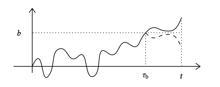
We consider the first arrivial time of position \(b\) in a Brownian motion. This is called the hitting time of \(b\). Define \[ \tau_b := \inf \left\{ t \geq 0 \mid W(t) > b \right\} \] For any \(t>0\), \[\begin{align*} \Pr{\tau_b \le t} &= \Pr{\tau_b \le t \wedge W(t) \le b} + \Pr{\tau_b \le t \wedge W(t) > b}\\ &= \Pr{W(t) > b} + \Pr{ W(t) \le b\mid \tau_b \le t }\cdot \Pr{\tau_b \le t }. \end{align*}\]

Note that \(W(t) \sim N(0,t)\). Let \(\Phi\) be the CDF of the standard Gaussian distribution. That is, \(\Phi(x) = \frac{1}{\sqrt{2\pi}} \int_{-\infty}^{x} e^{-\frac{t^2}{2}}dt\). Then \[ \Pr{W(t) > b} = \Pr{\frac{W(t)}{\sqrt{t}} > \frac{b}{\sqrt{t}}} = 1 - \Phi\tp{\frac{b}{\sqrt{t}}}. \]

Assuming we have known the value of \(\tau_b\) and \(\tau_b < t\), we can regard \(\set{W(t)}_{t\geq \tau_b}\) as a Brownian motion starting from \(b\). Thus, as the following figure shows, \(\Pr{ W(t) \le b\mid \tau_b \le t } = 1/2\). This is called the principle of reflection of a standard Brownian motion.

Substituting the above results into the original formula yields:

\[ \Pr{\tau_b \le t} = 2 \tp{ 1 - \Phi\tp{\frac{b}{\sqrt{t}}}}. \]