Lecture 6: Diffusions and Itô Calculus
Diffusion
In this lecture, we introduce a class of continuous-time stochastic processes known as diffusion processes.
Actually, diffusions can be built up from local Brownian motions in the same way as differentiable functions being built up from local linear functions. Imagine that we want to draw the image of a function \(f\) with knowing \(f'(t)=e^t\) and \(f(0)=1\). How to do this if you are not allowed to integrate \(f'(t)\). A natural idea is to approximate \(f\) using segmented linear functions:
- Select a step length \(h\);
- Draw a segment on \([0,h]\) which starts from \(\tp{0,f(0)}\) with slope \(f'(0)=1\);
- Draw a segment on \([h,2h]\) which starts from \(\tp{h,h+f(0)}\) with slope \(f'(h)=e^h\);
- \(\dots\)
When \(h\to 0\), our drawing is exactly the image of \(f\). This gives an intuition that a differentiable function can be locally approximated as linear functions.
A diffusion \(\set{X(t)}_{t\geq 0}\) is the stochastic analog of above process. It replaces the “local linear behavior” with “local Brownian motion”. That is, if we are currently at the position \(X(t) = X_t\) and consider the small time interval \([t,t+h]\), the increment \(X(t+h) - X(t)\) behaves like a normal random variable. Let \(Z_1,Z_2\dots\) be independent standard Gaussians. We can break the process into segments and use these normal random variables to simulate the diffusion:
- \(X_h=X_0+\mu(0,X_0)h+\sigma(0,X_0)\sqrt{h}\cdot Z_1\);
- \(X_{2h}=X_h+\mu(h,X_h)h+\sigma(h,X_h)\sqrt{h}\cdot Z_2\);
- \(\dots\)
where \(\mu\) and \(\sigma^2\) are functions of the time \(t\) and position \(X_t\). For any \(k\in\bb N\), \(X_{(k+1)h}-X_{kh}\sim\+N\tp{\mu(kh, X_{kh})h, \sigma^2(kh, X_{kh})h}\). Then for a diffusion \(\set{X(t)}_{t\geq 0}\) specified by \(\mu(t,x)\) and \(\sigma^2(t,x)\), we can write it as \[ \d X(t)=\mu(t,X(t))\d t+\sigma(t,X(t))\d B(t) \tag{1}\] where \(\set{B(t)}\) is the standard Brownian motion and \(\d B(t)\) can be understood as \(\lim_{h\to 0}B(t+h)-B(t)\).
The standard Brownian motion itself is a special diffusion process with \(\mu(t,x)\equiv 0\) and \(\sigma(t,x)\equiv 1\). Here are two other important examples.
Example 1 (Ornstein-Uhlenbeck process, OU process) Consider a diffusion \(\set{X(t)}_{t\geq 0}\) specified by \(\mu(t,x)=-x\) and \(\sigma^2(t,x)=2\) with \(X(0)=0\). This diffusion always has a tendency to \(0\) since if \(X(t)\) is large, \(\mu(t,X(t))\) is also large towards the reverse direction which acts as a spring intuitively. We can write this process as \[ \d X(t)=-X(t)\d t+\sqrt{2}\d B(t). \] The process can be used to model the discrete Ehrenfest chain. Suppose we have two boxes with \(a\) balls in the first box and \(b\) balls in the second box in the initial state. In each round, we choose a ball uniformly at random among the \(a+b\) balls and put the chosen ball into the other box. It is more likely to choose the balls in the box with more balls. Thus, this discrete Markov process tends to the equilibrium state where each box has \(\frac{a+b}{2}\) balls.
The OU process is a special case of the more general Langevin diffusion.
Example 2 (Langevin diffusion) To understand it, first recall the gradient descent algorithm. To minimize a function \(f(x)\), we follow the direction of the negative gradient: \[ X_{k+1} = X_k - \eta \nabla f(X_k), \] where \(\eta>0\) is the step size. This is a discrete approximation of the gradient flow differential equation, \(\d X(t) = -\nabla f(X(t)) \d t\), which deterministically follows paths of steepest descent to a local minimum of \(f\).
The Langevin diffusion adds a stochastic noise term to this flow: \[ \d X(t) = -\nabla f(X(t)) \d t + \sqrt{2}\d B(t). \] This process no longer just finds a single local minimum. Instead, the noise term allows the process to “jump out” of local minima and explore the entire state space. It can be shown that this process does not converge to a single point, but rather converges in distribution to a stationary distribution \(p(x)\) given by: \[ p(x) \propto e^{-f(x)}. \]
Itô Integral
Our informal SDE notation Equation 1 is convenient, but to work with it mathematically, we must express it in an integral form.
Given an ordinary differential equation \(\d f(t)=f(t)\d t\), we have that, \[ \forall T,\ \int_0^T\d f(t)=\int_0^Tf(t)\d t, \] which is equivalent to \[ \forall T,\ f(t)=f(0)+\int_0^Tf(t)\d t. \] If we apply the same process to Equation 1, we have that \[ \forall T,\ X(T)=X(0)+\int_0^T\mu\tp{t,X(t)}\d t+\int_0^T\sigma\tp{t,X(t)}\d B_t. \] Just to keep the notation simple, we’ll use \(X_t\) and \(X(t)\) interchangeably from now on, as long as it’s clear from the context. To be precise, for any specific outcome \(\omega\) in our probability space, this equation must hold for the realized paths:
\[ \begin{align*} X_t\tp{\omega}=X_0\tp{\omega}+\int_0^T\mu\tp{t,X_t\tp{\omega}}\d t+\int_0^T\sigma\tp{t,X_t\tp{\omega}}\d B_t\tp{\omega}. \end{align*} \]
We will omit the \(\omega\) in the following part if the context is clear. Note that \(\int_0^T\mu\tp{t,X_t}\d t\) is the ordinary Riemann integral of \(\mu\tp{t,X_t}\). The main goal today is to rigorously define the meaning of \(\int_0^T\sigma\tp{t,X_t}\d B_t\).
This cannot be defined as a standard Riemann-Stieltjes integral. When we use the notation \(\d F(t)\), we usually assume that function \(F\) is differentiable. However, \(\{B_t\}_{t\ge 0}\) is a stochastic process and nowhere differentiable. This “roughness” is what prevents standard integration from working and is why a new theory is required.
To see why is \(B_t\) not differentiable, recall that for a Brownian motion \(\set{B(t)}_{t\geq 0}\), the process \(\set{X(t)}_{t\geq 0}\) with \(X(t) = t\cdot B(1/t)\) is also a standard Brownian motion. Now, look at the definition of the derivative of \(B_t\) at \(t=0\): \[ \lim\sup_{t\to 0^+} \frac{B_t-B_0}{t} = \lim\sup_{t\to \infty} X(t). \] By the properties of Brownian motion, we know that \(\limsup_{s \to \infty} X(s) = \infty\) almost surely. Therefore, the derivative of \(B_t\) at \(t=0\) does not exist.
Quadratic variation
To give a formal definition of the diffusion, we review the concept of functions of bounded variation and introduce the definition of quadratic variation.
In standard calculus, we can integrate with respect to functions that are “well-behaved,” meaning they don’t oscillate infinitely. For a function \(f\) defined on the interval \([a,b]\), let \[ V_f([a, b]) = \sup \left\{ \sum_{i=0}^{n-1} |f(t_{i+1}) - f(t_i)| : a = t_0 < t_1 < \cdots < t_n = b \right\}, \] be the variation of \(f\). Note that if \(f\) is continuously differentiable, this is just \(V_f([a, b]) = \int_a^b |f'(t)| \d t\). If \(V_f([a, b]) < \infty\), we say \(f\) is of bounded variation.
However, for a typical sample path \(B_t(\omega)\) of Brownian motion, it is a known (and non-trivial) fact that \(V_{B_t(\omega)}([0, T]) = \infty\) almost surely. The path is of unbounded variation, so standard integration theories fail. While the sum of absolute changes diverges, the variance of Brownian motion, \(\E{(B_t - B_s)^2} = t-s\), scales nicely with time. This suggests that summing the squares of the increments might be more stable. This motivated us to define the notion of quadratic variation.
Definition 1 (Quadratic Variation) For a function \(f:[a,b]\to \bb R\), the quadratic variation is defined as
\[ Q_f([a,b]) = \lim_{\max \abs{t_i-t_{i-1}}\to 0} \set{\sum_{i=1}^n \tp{f(t_i) - f(t_{i-1})}^2 \mid a\leq t_0\leq t_1\cdots\leq t_n\leq b}. \]
We assume the limit exists almost surely for our informal development.
Denote \(Q_f([0,T])\) as \(Q_f(T)\) for simplification. Let’s compute this value for a standard Brownian motion \(\set{B_t}\) on \([0,T]\).
Let \(\Delta_i = t_i-t_{i-1}\). We first provide an informal derivation. In the following calculations, we always assume it is valid to swap integrals and limits (for our informal development). Then the expectation of \(Q_{B_t}(T)\) satisfies, \[ \begin{align*} \E{Q_{B_t}(T)} &= \lim_{\max \Delta_i\to 0} \sum_{i=1}^n \E{\tp{B(t_i) - B(t_{i-1})}^2}\\ \mr{$B(t_i) - B(t_{i-1})\sim \+N(0,\Delta_i)$}&= \lim_{\max \Delta_i\to 0} \sum_{i=1}^n \Delta_i\\ &=T. \end{align*} \] We can similarly compute its variance: \[ \begin{align*} \Var{Q_{B_t}(T)} &= \lim_{\max \Delta_i\to 0}\sum_{i=1}^n\Var{\tp{B_{t_i}-B_{t_{i-1}}}^2}\\ &= \lim_{\max \Delta_i\to 0} \tp{\sum_{i=1}^n\E{\tp{B_{t_i}-B_{t_{i-1}}}^4}-\sum_{i=1}^n\E{\tp{B_{t_i}-B_{t_{i-1}}}^2}^2}\\ &=2\lim_{\max \Delta_i\to 0} \sum_{i=1}^n \Delta_i^2\\ &\leq 2\lim_{\max \Delta_i\to 0} \tp{\max_{i\in[n]}\Delta_i}\cdot \sum_{i=1}^n \Delta_i\\ &=0. \end{align*} \]
We also include a formal proof of this result. The following lemma shows that \(\sum_{i=1}^n \tp{B(t_i)-B(t_{i-1})}^2\) converges to \(T\) in \(L^2\) (See the definition of convergence in \(L^2\) here).
Lemma 1 \[ \lim_{\max t_{i}-t_{i-1} \to 0} \E{\tp{\sum_{i=1}^n \tp{B(t_i)-B(t_{i-1})}^2 - T}^2} = 0. \]
Riemann-Stieltjes Integral
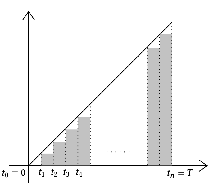
Consider the simple integral \(\int_0^T x\dd x\). As the following figure shows, we divide \([0,T]\) into \(n\) disjoint segments \([0,t_1],(t_1,t_2],\dots,(t_{n-1},T]\). Let \(\Delta_{i}=t_i-t_{i-1}\) and \(\Delta=\max_{i\in[n]} \Delta_{i}\). Then \[ \begin{align*} \int_0^T x\dd x&=\lim_{\Delta\to 0} \sum_{i=1}^n t_{i-1}(t_i-t_{i-1}) = \lim_{\Delta\to 0} -\frac{1}{2}\sum_{i=1}^n (t_i-t_{i-1})^2 + \frac{1}{2}\sum_{i=1}^n (t_i^2 - t_{i-1}^2). \end{align*} \]
Note that \(\sum_{i=1}^n (t_i^2 - t_{i-1}^2) = T^2\) and \[ \sum_{i=1}^n (t_i-t_{i-1})^2 \leq \tp{\max_{j\in[n]} \Delta_{j}}\cdot \sum_{i=1}^n (t_i-t_{i-1}) = \tp{\max_{j\in[n]} \Delta_{j}}\cdot T\to 0. \] Therefore, we have \(\int_0^T x\dd x=\frac{T^2}{2}\).
Let \(F\colon[0,T]\to \mathbb{R}\) be a function with bounded derivative. We can use the same idea to calculate \(\int_0^T F(x)\dd F(x)\): \[ \begin{align*} \int_0^T F(x)\dd F(x) &= \lim_{\Delta\to 0}\sum_{i=1}^n F(t_{i-1})\tp{F(t_i)-F(t_{i-1})} \\ &= \frac{1}{2}\tp{F(T)^2-F(0)^2} -\lim_{\Delta\to 0} \frac{1}{2}\sum_{i=1}^n \tp{F(t_i)-F(t_{i-1})}^2. \end{align*} \] If the derivative of \(F\) is bounded by \(M\) on \([0,T]\), we have \[ \begin{align*} \lim_{\Delta\to 0}\sum_{i=1}^n \tp{F(t_i)-F(t_{i-1})}^2 &\leq \lim_{\Delta\to 0}\tp{\max_{j\in[n]}\abs{F(t_j)-F(t_{j-1})} }\cdot \sum_{i=1}^n\abs{\tp{F(t_i)-F(t_{i-1})}}\\ &\leq \lim_{\Delta\to 0}\tp{\max_{j\in[n]}\abs{F(t_j)-F(t_{j-1})} }\cdot \sum_{i=1}^n M\cdot\tp{t_i-t_{i-1}}\\ &=\lim_{\Delta\to 0}\tp{\max_{j\in[n]}\abs{F(t_j)-F(t_{j-1})} }\cdot MT = 0. \end{align*} \]
Itô Integral
Consider what will happen if we substitute \(F\) with the standard Brownian motion \(\set{B_t}\). We can also deduce that \[ \int_0^T B_t\dd B_t = \frac{1}{2}B_T^2 - \frac{1}{2}\lim_{\Delta\to 0}\sum_{i=1}^n \tp{B_{t_i}-B_{t_{i-1}}}^2. \]
However, the quadratic variation \(\lim_{\Delta\to 0}\sum_{i=1}^n \tp{B_{t_i}-B_{t_{i-1}}}^2\) is no longer \(0\) but \(T\). Therefore, \[ \int_0^T B_t\dd B_t = \frac{1}{2}B_T^2 - \frac{T}{2}. \]
Definition 2 (Itô Integral.) Assume that \(\set{X_t}_{t\geq 0}\) is a “nice enough” stochastic process. Then we define the integral \(\int_0^T X_t\d B_t\) as the mean-square (\(L^2\)) limit of \[ \sum_{i=1}^nX_{t_{i-1}}\tp{B_{t_i}-B_{t_{i-1}}}. \tag 2 \] This is called the Itô integral of \(\set{X_t}_{t\geq 0}\) with respect to \(\set{B_t}_{t\geq 0}\).
Here, “nice enough” means that \(X_t\) is part of the information available up to time \(t\) (\(\mathcal{F}_t\)-measurable) and does not peek into the future. Some other technical requirements can be found in any standard textbook on stochastic differential equations (e.g. Introduction to stochastic calculus with applications).
This choice of the left-point \(X_{t_{i-1}}\) in Equation (2) is crucial. Because \(X_{t_{i-1}}\) is non-anticipating, it is independent of the future increment \((B_{t_{i}} - B_{t_{i-1}})\). This independence gives the Itô integral an important property: it is a martingale (under certain conditions).
More generally, we may define \(\int_0^T X_t\d B_t\) as the mean square limit of \[ \sum_{i=1}^n X_{t_i^*} \tp{B_{t_i}-B_{t_{i-1}}}, \] for \(t_i^*=\alpha\cdot t_{i-1}+(1-\alpha)\cdot t_i\) with \(\alpha\in[0,1]\). The Itô integral corresponds to the case that \(\alpha=1\). By choosing \(\alpha=\frac{1}{2}\), we have the definition of Stratonovich integral and it holds that \(\int_0^T B_t\d B_t=\frac{1}{2}B_T^2\) with Stratonovich integral
Since we can define integrals for all \(\alpha\in[0,1]\), it is natural to ask which value of \(\alpha\) produces the “correct” one? Actually, the best choice of \(\alpha\) depends on how you want to model the stochastic process. For example, when we view a diffusion \(\set{X_t}\) as the limit of a certain discrete process, the motion during \([t,t+h]\) for a tiny \(h\) is specified by \(\mu(t,X_t)\) and \(\sigma(t,X_t)\). So it is reasonable to specify a diffusion with Itô integral. However, for many stochastic processes from physics which are continuous in nature, it turns out that Stratonovich integral fits better.
Itô Formula
Recall that \[ \begin{align*} Q_{B_t}(T) &= \lim_{\max \abs{t_i-t_{i-1}}\to 0} \set{\sum_{i=1}^n \tp{B(t_i) - B(t_{i-1})}^2 \mid a\leq t_0\leq t_1\cdots\leq t_n\leq b}=T. \end{align*} \] We can write this identity heuristically using infinitesimal notation. If we think of \(\d B_t\) as an increment \((B_{t+\d t} - B_t)\), then the sum \(\sum (\d B_t)^2\) becomes an integral \(\int_0^T (\d B_t)^2\). This gives the remarkable heuristic identity:
\[ \int_0^T (\d B_t)^2 = T = \int_0^T \d t \quad \implies \quad (\d B_t)^2 \approx \d t. \]
With this observation, we then (heuristically) deduce the chain rule under the definition of Itô integral.
The classical chain rule
For any differentiable function \(f\), we have \(\dd f(t)=f'(t)\dd t\). This can be verified via Taylor’s expansion: \[ \begin{align*} \dd f(t) &= f(t+\dd t)-f(t) = f'(t)\dd t + \frac{1}{2}f''(t)\tp{\dd t}^2 + o\tp{(\dd t)^2}\overset{\dd t\to 0}{\to} f'(t)\dd t. \end{align*} \]
For two differentiable functions \(g\) and \(f\), the chain rule of differentiation is \[ \frac{\d f\tp{g(t)}}{\d t}=f'\tp{g(t)}\cdot g'(t). \] We can also derive this using the Taylor expansion: \[ \begin{align*} \d f\tp{g(t)}&=f\tp{g(t+\d t)}-f\tp{g(t)}\\ &=f\tp{g(t)+\d g(t)}-f\tp{g(t)}\\ &=f'\tp{g(t)}\d g(t)+\frac{1}{2}f''\tp{g(t)}\tp{\d g(t)}^2+o(\tp{\d g(t)}^2). \end{align*} \] Then it follows that \[ \frac{\d f\tp{g(t)}}{\d t}=f'\tp{g(t)}\cdot g'(t)+o(\d t)\overset{\dd t\to 0}{\to}f'\tp{g(t)}\cdot g'(t). \]
The chain rule with Itô Integral
Consider a diffusion \(\set{X_t}\) that \[ \d X_t=\mu_t\d t+\sigma_t\d B_t, \] where \(\mu_t\) and \(\sigma_t\) are the abbreviations of \(\mu(t,X_t)\) and \(\sigma(t,X_t)\) respectively. By the Taylor’s expansion, \[ \begin{align*} \d f\tp{X_t}&=f\tp{X_t+\d X_t}-f\tp{X_t}\\ &=f'\tp{X_t}\d X_t+\frac{1}{2}f''\tp{X_t}\tp{\d X_t}^2 + o\tp{\tp{\dd X_t}^2}\\ &= f'\tp{X_t}\tp{\mu_t\d t+\sigma_t\d B_t} + \frac{1}{2}f''\tp{X_t} \tp{\mu_t\d t+\sigma_t\d B_t}^2 + o\tp{\tp{\dd X_t}^2} \\ &\overset{\dd t\to 0}{\longrightarrow}\tp{f'\tp{X_t}\mu_t + \frac{1}{2}f''\tp{X_t}\sigma_t^2} \d t+f'\tp{X_t}\sigma_t\d B_t \end{align*} \] This chain rule with Itô integral is called Itô formula. Then we see some examples of Itô formula.
Example 3 We can use Itô formula to calculate \(B_T^2\). Note that \[ \d\tp{B_t}^2 = 2B_t\d B_t + \tp{\d B_t}^2 \] Therefore, \(B_T^2 = 2\int B_t\d B_t + T\).
Example 4 (Geometric Brownian motion) The geometric Brownian motion is \(Y_t=e^{B_t}\) where \(\set{B_t}\) is the standard Brownian motion. Then it follows from the Itô formula that \[ \begin{align*} \d Y_t=e^{B_t}\tp{\d B_t+\frac{1}{2}\tp{\d B_t}^2}=Y_t\d B_t+\frac{1}{2}Y_t\d t. \end{align*} \]
Example 5 (Ornstein-Uhlenbeck process) Let \(\set{X_t}\) be the Ornstein-Uhlenbeck process that \(\d X_t=-X_t\d t+2\d B_t\). We can calculate \(X_t\) according to this equation. Let \(f(t,X_t)=e^{t}\cdot X_t\). Using Taylor expansion, we have \[ \begin{align*} \d f(t,X_t)&=f(t+\d t,X_{t+\d t})-f(t,X_t)\\ &=X_te^t\dd t + e^t\d X_t\\ &=X_te^t\dd t-e^t\cdot X_t\d t+2e^t\d B_t = 2e^t\d B_t. \end{align*} \] Then we have \(e^TX_T - X_0=\int_0^T 2e^t\d B_t\) and \(X_T= e^{-T}X_0 + e^{-T}\int_0^T 2e^t\d B_t\). Since \(\int_0^T 2e^t\d B_t\) can be viewed as the limit of the weighted sum of many Gaussian random variables, one can verify that \(\int_0^T 2e^t\d B_t\sim \+N\tp{0,4\int_0^T e^{2t}\d t}\). This shows that the distribution of \(X_T\) can be viewed as a Gaussian centered at the decaying initial condition.