Lecture 9: Tensorization of Entropy, the Modified Log-Sobolev inequality

Author

instructed by Chihao Zhang, scribed by Yuxuan Wang and Yuchen He

In our last lecture, we explored the tensorization of variance and generalized it to the Poincaré inequality in the context of Markov processes: \[ \forall f,\ \Var[\pi]{f}\leq c\cdot \+{E}(f,f). \] We also established several equivalent characterizations of this inequality, including:

Variance decay: The variance of the evolved function contracts exponentially: \[ \Var[\pi]{P_t f}\leq e^{-\frac{2t}{c}}\cdot \Var[\pi]{f}. \]

If we let $f=\frac{\d \mu_0}{\d \pi}$ (the density ratio of the initial distribution $\mu_0$ with respect to the stationary measure $\pi$), this variance contraction directly implies the convergence of the $\chi^2$-divergence: \[ \chi^2(\mu_t\| \pi)\defeq \int_{\Omega} \left(\frac{\d\mu_t}{\d\pi}-1\right)^2 \d\pi \leq e^{-\frac{2t}{c}}\cdot \chi^2(\mu_0\| \pi). \]

Dirichlet form contraction: The energy of the function dissipates exponentially:\[\mathcal{E}(P_t f, P_t f)\leq e^{-\frac{2t}{c}}\mathcal{E}(f,f).\]We proved that this one-step contraction is sufficient to imply the Poincaré inequality.

The Poincaré inequality establishes a vital link between the concentration of measure and the convergence of Markov processes. However, it has a limitation. By controlling the variance, it only guarantees polynomial concentration and is insufficient to capture the exponential concentration (e.g., sub-Gaussian tails) frequently observed in high-dimensional probability. To derive these sharper bounds and to analyze the convergence of Markov processes toward such strongly concentrated stationary distributions, we require a more powerful tool than the Poincaré inequality. In this lecture, we will introduce the modified log-Sobolev inequality (MLSI).

Tensorization of entropy

As before, we consider a random vector $X=(X_1,\dots,X_n)\in \mathbb{R}^n$ and a function $f:\mathbb{R}^n\to \mathbb{R}$.Recall McDiarmid’s inequality. Assuming $X_i$’s are mutually independent, then for any $t>0$, \[ \Pr{f(X)-\E{f(X)}\geq t} \leq \exp\left\{-\frac{2t^2}{\sum_{i=1}^n (b_i-a_i)^2}\right\}, \] where the sensitivity parameter is defined as \[ b_i-a_i = \sup_{x\in \mathbb{R}^n} \left| \sup_{z\in \mathbb{R}} f(x_{-i}, z) - \inf_{z\in \mathbb{R}} f(x_{-i}, z) \right|. \] This notion of tensorization is in a sense weak. We can compare it to the tensorization of variance we studied previously: \[ \Var[\pi]{f} \lesssim \E[\pi]{\sum_{i=1}^n \tp{\mbox{gradient}_i(f)}^2}. \] Notice the key difference: the $b_i-a_i$ term in McDiarmid’s inequality represents the maximum sensitivity (the worst-case over all $x\in \mathbb{R}^n$) of the $i$-th coordinate, whereas the variance bound relies on the expected sensitivity. This observation motivates the following questions:

Can we obtain better concentration characterizations for $f(X)$ than McDiarmid’s inequality without relying on the worst-case sensitivity, at least the worst-case for each coordinate?
Can we prove tensorization formulas for a different quantity that captures stronger concentration properties (such as sub-Gaussian tails) and use it to characterize the convergence of Markov processes?

Characterizing Sub-Gaussianity via Entropy

We begin by examining sub-Gaussian random variables. Recall that a random variable $X\in \mathbb{R}$ is called $c^2$-sub-Gaussian if \[ \forall \lambda\in \bb R,\ \psi(\lambda) \defeq \log \E{e^{\lambda(X-\E{X})}}\leq \frac{c^2}{2}\cdot \lambda^2. \] This is equivalent to requiring $\frac{\psi(\lambda)}{\lambda}\leq \frac{c^2}{2}\lambda$. Essentially, the sub-Gaussian property asserts that the moment generating function (MGF) is well-behaved. However, the MGF itself does not tensorize easily. To address this, we seek an equivalent characterization of the sub-Gaussian property that is amenable to tensorization.

In statistical physics, the quantity $\frac{\psi(\lambda)}{\lambda}$ is known as the negative free energy. Let us compute its derivative with respect to $\lambda$: \[ \begin{align*} \frac{\d}{\d \lambda} \frac{\psi(\lambda)}{\lambda} &= \frac{\d}{\d \lambda}\tp{\frac{\log \E{e^{\lambda X}}}{\lambda} - \E{X}}\\ &=\frac{1}{\lambda^2}\cdot \tp{\lambda\cdot \frac{\E{Xe^{\lambda X}}}{\E{e^{\lambda X}}} - \log \E{e^{\lambda X}}}\\ &= \frac{1}{\lambda^2}\cdot \frac{\E{\lambda X\cdot e^{\lambda X}} - \E{e^{\lambda X}}\log \E{e^{\lambda X}}}{\E{e^{\lambda X}}}. \end{align*} \]

To interpret the numerator, we introduce the concept of $\phi$-entropy. For a convex function $\phi:\mathbb{R}\to \mathbb{R}$, we define the $\phi$-entropy of a random variable $Z$ as: \[ \phi\mbox{-}\Ent{Z} \defeq \E{\phi(Z)} - \phi\tp{\E{Z}}. \] When $\phi(x)=x^2$, this corresponds to the variance. When $\phi(x)=x\log x$, it is called the entropy and denoted simply as $\Ent{Z}$. To see why this is called entropy, let $\bb P$ and $\bb Q$ be two probability measures with $\bb P \ll \bb Q$. Consider the likelihood ratio $Z=\frac{\d \bb P}{\d \bb Q}(X)$ with $X\sim \bb Q$. Then \[ \Ent{Z} = \E[X\sim \bb Q]{\frac{\d \bb P}{\d \bb Q}(X)\cdot \log \frac{\d \bb P}{\d \bb Q}(X)} = \E[X\sim \bb P]{\log \frac{\d \bb P}{\d \bb Q}(X)} = \!{KL}(\bb P\|\bb Q). \] This recovers the relative entropy (or equivalently, Kullback-Leibler (KL) divergence) between $\bb P$ and $\bb Q$.

With this definition, we can rewrite the derivative of the negative free energy in a compact form: \[ \frac{\d}{\d \lambda} \frac{\psi(\lambda)}{\lambda} = \frac{1}{\lambda^2}\cdot \frac{\Ent{e^{\lambda X}}}{\E{e^{\lambda X}}}. \] This relationship implies that if we can bound the entropy, we can bound the free energy (by integration), and thus establish sub-Gaussianity. Specifically, \[ \Ent{e^{\lambda X}} \leq \frac{c^2\lambda^2}{2}\E{e^{\lambda X}} \] is a sufficient condition for $X$ to be $c^2$-sub-Gaussian.

In fact, this is also a necessary condition. If a distribution is $c^2$-sub-Gaussian, one can show that $\Ent{e^{\lambda X}} \leq \frac{O(c^2)\lambda^2}{2}\cdot \E{e^{\lambda X}}$ holds for any $\lambda$. Therefore, this entropy bound serves as a sufficient and necessary condition for the sub-Gaussian property.

Tensorization of entropy

Just as variance can be tensorized to prove the Poincaré inequality, entropy satisfies a similar tensorization property. Let us again consider a function $f(X)=f(X_1,\dots,X_n)$. Recall that in our study of the Poincaré inequality, our goal was to establish an inequality of the form: \[ \Var{f}\lesssim \E{\|\mbox{gradient} (f)\|^2}. \] Now, we aim to establish an analogous formula for entropy to characterize stronger concentration properties. Specifically, we want to prove that: \[ \Ent{e^{\lambda f}} \lesssim \E{\|\mbox{gradient} (\lambda f)\|^2 e^{\lambda f}}. \] This inequality is intimately connected to sub-Gaussian distributions. Notice that in the one-dimensional case where $n=1$ and $f(X)=X$, this inequality implies the sufficient condition for the sub-Gaussian property that we derived in the previous section.

Inequalities of this type are called modified log-Sobolev inequalities (MLSI). To establish the MLSI in high dimensions, we will follow a strategy of two steps:

Tensorization: Decompose the global entropy into a sum of local entropies.
Local bound: Derive a one-dimensional MLSI to bound each local term $\Ent[i]{f(X)}$.

We start with the tensorization theorem.

Theorem 1 (Tensorization of entropy) Suppose $X_1,\dots,X_n$ are mutually independent. Then \[ \Ent{f(X)} \leq \sum_{i=1}^n \E{\Ent[i]{f(X)}}, \] where $\Ent[i]{f(X)} = \Ent{f(X)\mid X_{-i}}$ and $X_{-i} = (X_1,\dots,X_{i-1},X_{i+1},\dots,X_n)$.

To prove this theorem, we first introduce the variational characterization of entropy.

The variational characterization of entropy

We will prove that for a non-negative random variable $Z$, the entropy $\Ent{Z}$ can be expressed as the solution to an optimization problem: \[ \Ent{Z} = \sup_{X}\set{\E{ZX}:\ \E{e^X}=1}. \] To derive this, we rely on convex duality. Recall that for a function $f:\mathbb{R}^d\to \mathbb{R}$, its Fenchel dual (or convex conjugate) is defined as: \[ f^*(z) =\sup_{x\in \bb R}\set{\inner{z}{x} - f(x)}. \]

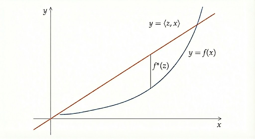
When $f$ is convex and lower semi-continuous, we have $(f^*)^* =f$. Consider the functional $F(Z) = \Ent{Z}$ defined on the space of non-negative random variables. Since the function $\phi(x) = x \log x$ is convex, it is easy to verify that $F(Z)$ is a convex function. Therefore, we can express entropy via its double conjugate: \[ \Ent{Z} = F(Z) = F^{**}(Z) = \sup_X\set{\E{ZX} - F^*(X)}. \] Our goal is to calculate the dual functional $F^*(X)$. Without loss of generality, let us first restrict our attention to the case where $\E{Z}=1$. In this case, $\Ent{Z}=\E{Z\log Z}$. By definition, the dual is:

\[ F^*(X) = \sup_{Z:\E{Z}=1\atop Z\geq 0} \set{\E{ZX} - \E{Z\log Z}}. \] We employ the method of Lagrange multipliers. We introduce a multiplier $\lambda$ for the constraint $\E{Z}=1$ and define the Lagrangian: \[ L(Z,\lambda) = \tp{\E{ZX} - \E{Z\log Z}} - \lambda\tp{\E{Z}-1}. \] Rearranging the terms, we have $L(Z,\lambda) = \E{ZX - Z\log Z - \lambda Z} + \lambda$. To maximize this pointwise, consider the scalar function $g(z) = zx - z\log z -\lambda z$. We find its critical point by setting the derivative to zero: \[ \frac{\d }{\d z}g(z) = x-\lambda - \log z -1 = 0. \] Solving for $z$, we obtain the optimal $z^*=e^{x-\lambda -1}$. Thus, the random variable $Z^*$ that maximizes the Lagrangian is $e^{X-\lambda-1}$. Furthermore, to satisfy the constraint $\E{Z^*} = 1$, we must have $\E{e^{X - \lambda - 1}} = 1$. Solving for $\lambda$ yields $\lambda = \log \E{e^X} - 1$.

Substituting $Z^*$ and $\lambda$ back into the expression for the dual, we have \[ F^*(X) = \E{Z^* X} - \E{Z^* \log Z^*} = \E{Z^*\tp{X-(X-\lambda -1)}} = \lambda +1 = \log \E{e^X}. \] This yields the Donsker-Varadhan variational formula for $Z$ satisfying $\E{Z}=1$: \[ \Ent{Z} = \sup_{X} \set{\E{ZX} - \log \E{e^X}}. \]

Finally, we extend this to a general non-negative random variable $Z$, where $\E{Z}$ is not necessarily $1$. Let $\widehat{Z} = \frac{Z}{\E{Z}}$. The entropy scales as follows: \[ \Ent{\wh Z} = \E{\wh Z\log \wh Z} = \frac{1}{\E{Z}}\tp{\E{Z\log Z} - \E{Z\log \E{Z}}} = \frac{\Ent{ Z}}{\E{Z}}. \] Substituting this into the Donsker-Varadhan formula: \[ \begin{align*} \Ent{Z} &= \E{Z}\cdot \sup_X\set{\E{\frac{Z}{\E{Z}}\cdot X} - \log \E{e^X}}\\ &=\sup_X\set{\E{Z X} - \E{Z}\log \E{e^X}} \end{align*} \] Notice that the expression inside the supremum is invariant under shifting $X$ by a constant. Therefore, we can restrict the search space to those $X$ satisfying the normalization $\E{e^X}=1$. This gives us the final form: \[ \Ent{Z} = \sup_{X:\E{e^X}=1}\set{\E{ZX}}. \]

Proof of the tensorization of entropy

We now provide a proof of the tensorization theorem using martingale techniques. Let $f(X)$ be a non-negative function. Consider the Doob martingale $Z_k = \E{f(X)\mid \mathcal{F}_k}$, where $\mathcal{F}_k=\sigma(X_1,\dots,X_k)$ is the filtration generated by the first $k$ variables. Instead of the standard difference sequence, we define the increments in the logarithmic domain: $U_k=\log Z_k - \log Z_{k-1}$. Then we can expand the entropy using a telescoping sum: \[ \Ent{f(X)} = \E{Z_n\cdot \tp{\log Z_n - \log \E{Z_n}}} = \sum_{k=1}^n \E{Z_n\cdot U_k}. \] To bound each term $\E{Z_n \cdot U_k}$, we use the variational characterization. Let us examine the conditional expectation of $e^{U_k}$ given all variables except $X_k$. Let $\mathcal{F}_{-k} = \sigma(X_1, \dots, X_{k-1}, X_{k+1}, \dots, X_n)$. Note that $e^{U_k} = \frac{Z_k}{Z_{k-1}}$. Since the $X_i$’s are mutually independent, averaging over $X_k$ conditioned on $\mathcal{F}_{-k}$ yields: \[ \E{e^{U_k}\mid \+F_{-k}} = \E{\frac{Z_k}{Z_{k-1}}\mid \+F_{-k}} = \frac{\E{ \E{f\mid \+F_k}\mid \+F_{-k}}}{\E{f\mid \+F_{k-1}}} = 1. \] Now we apply the variational characterization of entropy. We have \[ \E{Z_n\cdot U_k\mid \+F_{-k}}\leq \Ent{Z_n\mid \+F_{-k}} = \Ent[k]{f}. \] Summing over $k=1$ to $n$ completes the proof.

The modified log-Sobolev inequality

Recall that our goal is to establish a modified log-Sobolev inequality of the form: \[ \Ent{e^{\lambda f}}\lesssim \E{\|\mbox{gradient} (\lambda f)\|^2 e^{\lambda f}}. \] Having proven the tensorization theorem, our strategy is to prove this inequality for the 1-dimensional case and then lift it to high dimensions. Specifically, for a scalar random variable $X \in \mathbb{R}$ and a function $h:\mathbb{R}\to \mathbb{R}$, we aim to bound the entropy of $e^{h(X)}$ using a term related to the gradient of $h$.

Lemma 1 (1-dimensional MLSI) We have \[ \Ent{e^h} \leq \!{Cov}(h,e^h) \leq \E{|D^{-}h|^2\cdot e^h}, \] where $D^{-}h(x) = h(x) - \inf h$.

Proof. For the first inequality, \[ \begin{align*} \Ent{e^h} &= \E{h\cdot e^h} - \E{e^h}\cdot \log \E{e^h}\\ \mr{Jensen's inequality}&\leq \E{h\cdot e^h} - \E{e^h}\cdot \E{h}\\ &=\!{Cov}(h,e^h). \end{align*} \] For the second inequality, \[ \begin{align*} \!{Cov}(h,e^h) &= \E{(h-\E{h})\cdot \tp{e^h -\E{e^h}}}\\ \mr{$\E{e^h -\E{e^h}}=0$}&= \E{(h-\inf h)\cdot \tp{e^h -\E{e^h}}}\\ &\leq \E{(h-\inf h)\cdot \tp{e^h -e^{\inf h}}}\\ &\leq \E{(h-\inf h)\cdot e^h\cdot (h-\inf h)}. \end{align*} \] This completes the proof.

We can now combine this 1-dimensional lemma with the tensorization of entropy to derive concentration bounds for high-dimensional functions $f:\mathbb{R}^n\to \mathbb{R}$ on independent variables $X=(X_1,\dots,X_n)$. Applying the tensorization theorem and the lemma to each coordinate $i$ (with $h = \lambda f$): \[ \begin{align*} \Ent{e^{\lambda f}} &\leq \sum_{i=1}^n \E{\Ent[i]{e^{\lambda f}}} \\ &= \lambda^2 \sum_{i=1}^n \E{(D_i f)^2 e^{\lambda f}} \end{align*} \] where $D_i f(x) = f(x) - \inf_{z} f(x_1, \dots, z, \dots, x_n)$. This gives the MLSI we want. And it further yields \[ \Ent{e^{\lambda f}}\leq \lambda^2 \cdot \max_{x\in \bb R^n} \sum_{i=1}^n \tp{D_i f}^2 \cdot \E{e^{\lambda f}}, \]

Comparing this to the sufficient condition for sub-Gaussianity, this inequality implies that the random variable $f(X)$ is sub-Gaussian with parameter $\sum_{i=1}^n \tp{D_i f}^2$. This gives the sub-Gaussian tail: for $t\geq 0$ \[ \Pr{f(X)-\E{f}\geq t} \leq \exp\set{-\frac{t^2}{4\norm{\sum_{i=1}^n \tp{D_i f}^2}_{\infty}}}, \] which is in general better than the McDiarmid’s inequality.

MLSI associated with Markov processes

We have demonstrated how to build MLSI for independent random variables using the tensorization theorem. Now we generalize it to the case where the variables can be dependent. We introduce the MLSI associated with Markov processes. Recall that for a Markov process with generator $\+L$ and stationary distribution $\pi$, the Dirichlet form $\+E(f,g)\defeq \inner{f}{\+L g}_{\pi}$.

Definition 1 (Modified log-Sobolev inequality) We say a Markov process with stationary distribution $\pi$ satisfies the modified log-Sobolev inequality with constant $c$ if for all functions $f$: \[ \Ent[\pi]{f} \leq c\cdot \mathcal{E}(\log f,f). \]

Analogous to the Poincaré inequality, the MLSI is equivalent to the exponential decay of entropy along the Markov process.

Theorem 2 For a Markov semigroup $\set{P_t}_{t\geq 0}$, the following statements are equivalent. 1, $\forall f,\ \Ent{f}\leq c\cdot \+E(\log f,f)$; 2. $\forall f,\ \Ent{P_tf}\leq e^{-\frac{t}{c}}\cdot \Ent{f}$; 3. $\forall f,\ \+E(\log P_t f,P_t f)\leq e^{-\frac{t}{c}}\cdot \+E(\log f,f)$;

The proof strategy is similar to that of the Poincaré inequality. Here, we demonstrate the implication $(3) \Rightarrow (1)$ to illustrate the connection between the dissipation of the Dirichlet form and the total entropy.

Proof (Proof of $(3) \Rightarrow (1)$). First, we calculate the time derivative of the entropy along the flow. We have \[\begin{align*} \frac{\d}{\d t}\Ent{P_tf} &= \E{\+L P_t f\log P_t f + \+L P_t f}. \end{align*}\] Since $\pi$ is the stationary distribution, \[ \E{\+L P_t f} = \int \left( \frac{\d}{\d t} P_t f(x) \right) \pi(x) \d x = \frac{\d}{\d t} \left( \int P_t f(x) \pi(x) \d x \right) = 0. \] Therefore, $\frac{\d}{\d t}\Ent{P_tf} = -\+E(\log P_t f, P_t f)$.

Assume (3) holds. We can recover the total entropy by integrating the derivative from $t=0$ to $\infty$ \[ \begin{align*} \Ent{f} &= -\int_0^{\infty} \frac{\d}{\d t}\Ent{P_tf}\d t \\ &= \int_0^{\infty}\+E(\log P_t f, P_t f)\d t\\ &\leq \int_0^{\infty}e^{-\frac{t}{c}}\cdot \+E(\log f,f) \d t\\ &\leq c\cdot \+E(\log f,f). \end{align*} \]

Comparison between the Poincare inequality and MLSI

While both the Poincaré inequality (PI) and the modified log-Sobolev inequality (MLSI) indicate exponential convergence of a Markov process, they differ in strength. In fact, the MLSI implies the Poincaré inequality: if a process satisfies MLSI with constant $c$, it also satisfies PI with the same constant $c$.

An significant advantage of MLSI lies in the metric of convergence it controls. Recall that if we choose $f=\frac{\d\mu_0}{\d\pi}$, the Poincaré inequality implies the exponential decay of the $\chi^2$-divergence: \[ \chi^2(\mu_t\|\pi) \leq e^{-\frac{t}{c}}\cdot \chi^2(\mu_0\|\pi). \] However, the initial error $\chi^2(\mu_0\|\pi)$ can be prohibitively large in high dimensional cases. Consider the random walk on the hypercube $\{\pm 1\}^n$. If the stationary distribution $\pi$ is uniform and we start from a fixed vertex (a point mass distribution), the initial divergence is: \[ \chi^2(\mu_0\|\pi) = \int \left(\frac{\d\mu_0}{\d\pi}\right)^2 \d\pi - 1 = \frac{1}{2^{-n}} - 1 \approx 2^n. \] Because the starting error is exponential in $n$, the time $t$ required to reduce the error to a constant is $\+O(n)$.

In contrast, MLSI controls the decay of entropy, which corresponds to the KL divergence. For the evolved density $f_t = P_t f = \frac{d\mu_t}{d\pi}$: \[ \Ent{P_t f} = \E[\mu_t]{\log \frac{\d\mu_t}{\d\pi}} = \!{KL}(\mu_t\|\pi). \] For the same starting condition (a point mass on the hypercube), the initial KL divergence is merely linear in $n$: \[ \!{KL}(\mu_0\|\pi) = \log \left(\frac{1}{2^{-n}}\right) = \log(2^n) = \+O(n). \] Because the starting error is only $\+O(n)$, the time required to dampen this error to a constant is only $\+O(\log n)$.

Let us now verify the MLSI for some specific examples.

Example 1 Consider a simple continuous-time Markov process defined as follows: starting from an initial distribution $X_0 \sim \mu_0$, events occur according to a Poisson process with rate $1$. When an event occurs, the state is effectively “reset” by sampling a new state $X_t$ from the stationary distribution $\mu$.

The transition operator $P_t$ for this process has a simple explicit form. For any function $f$: \[ P_t f(x) = e^{-t} f(x) + (1 - e^{-t}) \E{f}. \] Intuitively, with probability $e^{-t}$, no reset has occurred (the value remains $f(x)$), and with probability $1-e^{-t}$, at least one reset has occurred (the process has mixed completely to $\E{f}$). The generator is $\mathcal{L}f = \E{f} - f$. Therefore, the Dirichlet form is simply the covariance: \[ \mathcal{E}(f, g) = -\langle f, \mathcal{L}g \rangle_\pi = \E{f\cdot (g - \E{g})} = \operatorname{Cov}_\mu(f, g). \]

To establish the MLSI, we analyze the entropy for the evolved function $P_t f$: \[ \begin{aligned} \Ent{P_t f} &= \E{P_t f \log P_t f} - \E{P_tf} \log \E{P_tf} \\ \mr{Jensen's inequality}&\leq e^{-t} \E{f\log f} + (1-e^{-t})\E{f}\log \E{f}- \E{P_tf} \log \E{P_tf}\\ \mr{$\E{P_t f}=\E{f}$}&= e^{-t} \E{f\log f} + (1-e^{-t})\E{f}\log \E{f}- \E{f} \log \E{f}\\ &= e^{-t}\tp{\E{f\cdot \log f} -\E{f}\log \E{f} }\\ &= e^{-t}\cdot \Ent{f} \end{aligned} \] Recall that exponential decay $\Ent{P_t f} \leq e^{-t/c} \Ent{f}$ implies the MLSI with constant $c$. Thus, this process satisfies the MLSI with constant $c=1$: $\Ent{f} \le \+E(\log f, f)$.

Example 2 (MLSI for the standard Gaussian) We return to the OU process to establish the MLSI for the standard Gaussian distribution. Recall the key properties of the OU process: * $\mathcal{E}(f, g) = \E[\mu]{f'g'}$. * $P_t f(x) = \E{f(e^{-t}x+\sqrt{1-e^{-2t}} \xi)}$ where $\xi\sim \+N(0,1)$.

From the second property, we have $(P_t f)' = e^{-t} P_t(f')$. We then verify the condition (3) of the equivalence theorem. Note that \[ \begin{aligned} \+E(\log P_t f, P_t f)=\E{ (\log P_t f)'\cdot (P_t f)'} = \E{\dfrac{((P_tf)')^2}{P_t f}} = e^{-2t} \cdot \E{\frac{\tp{P_t(f')}^2}{P_tf}}. \end{aligned} \] Then we bound the term $\tuple {P_t (f')}^2$: \[\begin{aligned} (P_t f'(x))^2 &= \left( \E{f'(X_t) \mid X_0=x} \right)^2 \\ &= \left( \E{ \frac{f'(X_t)}{\sqrt{f(X_t)}} \cdot \sqrt{f(X_t)} \mid X_0=x } \right)^2 \\ \mr{Cauchy-Schwarz} &\le \E{\frac{(f'(X_t))^2}{f(X_t)} \mid X_0=x} \cdot \E{ f(X_t) \mid X_0=x } \\ &= P_t\left( f' \tp{\log f}'\right)(x) \cdot P_t f(x). \end{aligned}\]

Substituting this back into our expression: \[ \+E(\log P_t f, P_t f)\le e^{-2t} \cdot \E{P_t(f'(\log f)')}. \] Since $\E{P_t(f'(\log f)')} = \E{f'(\log f)'}$, we have \[ \+E(\log P_t f, P_t f)\leq e^{-2t} \cdot \E{f'(\log f)'} = e^{-2t} \cdot\+E\tp{\log f, f}. \] This establishes the contraction of the Dirichlet form with rate $e^{-2t}$ and thus implies that the standard Gaussian distribution satisfies the MLSI with constant $1/2$: \[ \Ent{f} \le \frac{1}{2}\cdot \+ E(\log f, f). \]

For the high dimensional Gaussian $X\sim \+N(0,I_d)$ in $\bb R^d$, we can derive its MLSI via the tensorization theorem. From the tensorization theorem, \[ \Ent{e^{\lambda f}} \le \sum_{i=1}^d \E{\Ent[i]{e^{\lambda f}} }. \] Since $X_i's$ are independent, the 1-dimensional MLSI gives \[ \Ent[i]{e^{\lambda f}}\leq \frac{\lambda^2}{2}\E{\frac{\partial f}{\partial x_i}\cdot \frac{\partial f}{\partial x_i}\cdot e^{\lambda f} \mid X_{-i}} \] Combining these formulas gives the MLSI for $\+N(0,I_d)$: \[ \Ent{e^{\lambda f}} \le \sum_{i=1}^d \E{\frac{\lambda^2}{2}\E{\tp{\frac{\partial f}{\partial x_i}}^2\cdot e^{\lambda f} \mid X_{-i}}} = \frac{\lambda^2}{2}\E{\norm{\nabla f}^2 e^{\lambda f}}. \] This further indicates that for $X\sim \+N(0,I_d)$ and for any $f$, $f(X)$ is $\max_{x} \|\nabla f\|^2$-sub-Gaussian.